
SLIDE 1 email
Subhransu Maji
November 3, 2016
CMPSCI 670: Computer Vision
Linear models
Subhransu Maji (UMASS) CMPSCI 670
A neuron (or how our brains work)
2
Neuroscience 101
Subhransu Maji (UMASS) CMPSCI 670
Input are feature values Each feature has a weight Sum in the activation If the activation is:
- > b, output class 1
- otherwise, output class 2
Perceptron
3
> b
Σ
w1 w2 w3 x3 x2
x1 activation(w, x) = X
i
wixi = wT x x → (x, 1) wT x + b → (w, b)T (x, 1)
Subhransu Maji (UMASS) CMPSCI 670
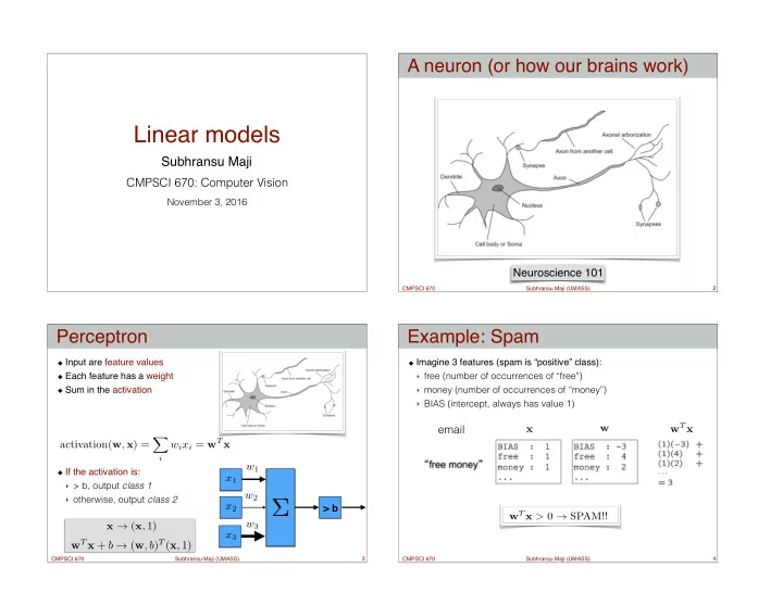
Imagine 3 features (spam is “positive” class):
- free (number of occurrences of “free”)
- money (number of occurrences of “money”)
- BIAS (intercept, always has value 1)
Example: Spam
4
w x wT x wT x > 0 → SPAM!!