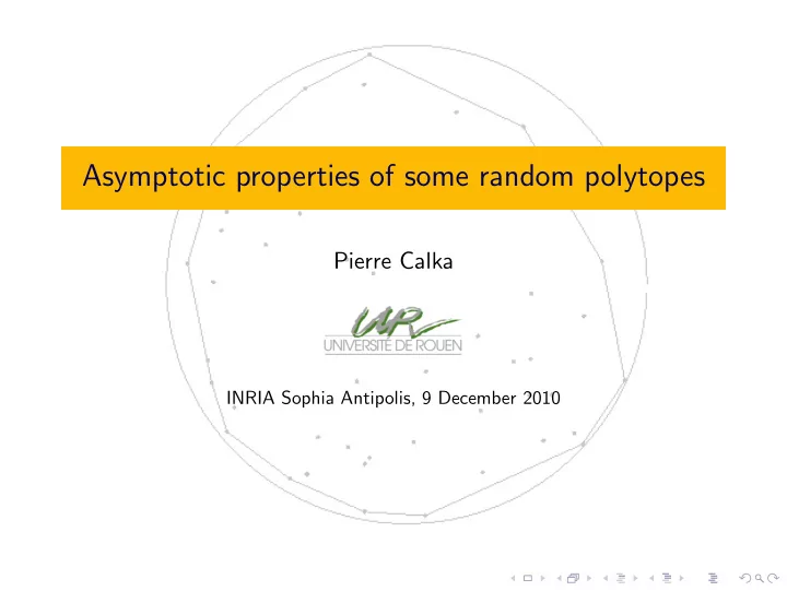
SLIDE 1
Asymptotic properties of some random polytopes
Pierre Calka
INRIA Sophia Antipolis, 9 December 2010
SLIDE 2
default
Outline
Random convex hulls in the unit-ball Random tessellations in Rd. Typical cell Convergence of the boundary and consequences Joint work with Tomasz Schreiber (Toru´ n University, Poland) and Joseph Yukich (Lehigh University, USA)
SLIDE 3
default
Outline
Random convex hulls in the unit-ball Poisson point process Model Historical background Random tessellations in Rd. Typical cell Convergence of the boundary and consequences
SLIDE 4 default
Poisson point process
B2 B3 B4
Poisson point process of intensity measure µ :=locally finite set X of Rd such that
◮ #(X ∩ B1) Poisson r.v. of mean µ(B1) ◮ #(X ∩ B1), · · · , #(X ∩ Bn) independent
(B1, · · · , Bn ∈ B(Rd), Bi ∩ Bj = ∅, i = j)
If µ = λdx, X homogeneous of intensity λ
SLIDE 5 default
Random convex hulls in the unit-ball
◮ X homogeneous Poisson point process in the unit-ball Bd of intensity λ > 0
(resp. set of n independent and uniform points)
◮ Convex hull Kλ (resp. K ′
n) of X
SLIDE 6 default
Historical background
Non-asymptotic results ◮ Sylvester (1864): four-point problem 2 3 ≤ pC ≤ 1 − 35 12π2
pC := probability that 4 i.i.d. uniform points in a convex set C ⊂ R2 are extreme
◮ Wendel (1962): P{0 ∈ K ′
n} = 2−(n−1) d−1
n − 1 k
◮ Efron (1965): f0(·):= # vertices, Vd(·):=volume, κd := Vd(Bd) κdEf0(K ′
n) = n
n−1)
- Buchta (2005): identities relating higher moments
SLIDE 7 default
Historical background
LLN
R´ enyi & Sulanke (1963), Wieacker (1978), Schneider & Wieacker (1980), Schneider (1988), B´ ar´ any & Buchta (1993)
κd − Vd(Kλ) ≈ cdλ−
2 d+1,
f0(Kλ) ≈ c′
dλ
d−1 d+1
CLT
Reitzner (2005), Vu (2006), Schreiber & Yukich (2008), B´ ar´ any & Reitzner (2009), B´ ar´ any et al. (2009)
Aims Description of the boundary of Kλ CLT with variance asymptotics
SLIDE 8
default
Outline
Random convex hulls in the unit-ball Random tessellations in Rd. Typical cell Poisson-Voronoi tessellations Poisson hyperplane tessellations Zero-cell and typical cell Distributional and asymptotic results Connection with random convex hulls Convergence of the boundary and consequences
SLIDE 9
default
Poisson-Voronoi tessellations
◮ X Poisson point process in Rd of
intensity measure dx
◮ For a nucleus x ∈ X, cell
C(x|X) := {y ∈ Rd : y − x ≤ y − x′ ∀x′ ∈ X}
◮ Tessellation: set of cells C(x|X)
Properties: isotropic, stationary, ergodic. References: Descartes (1644), Gilbert (1961), Okabe et al. (1992)
SLIDE 10
default
Poisson hyperplane tessellations
◮ X Poisson point process in Rd of
intensity measure xα−ddx (α ≥ 1)
◮ For x ∈ X, polar hyperplane
Hx := {y ∈ Rd : y − x, x = 0}
◮ Tessellation: set of connected
components of Rd \ ∪x∈XHx Properties: isotropic, stationary iff α = 1, ergodic. References: Meijering (1953), Miles (1964), Stoyan et al. (1987)
SLIDE 11
default
Poisson hyperplane tessellations
◮ X Poisson point process in Rd of
intensity measure xα−ddx (α ≥ 1)
◮ For x ∈ X, polar hyperplane
Hx := {y ∈ Rd : y − x, x = 0}
◮ Tessellation: set of connected
components of Rd \ ∪x∈XHx Properties: isotropic, stationary iff α = 1, ergodic. References: Meijering (1953), Miles (1964), Stoyan et al. (1987)
SLIDE 12
default
Poisson hyperplane tessellations
◮ X Poisson point process in Rd of
intensity measure xα−ddx (α ≥ 1)
◮ For x ∈ X, polar hyperplane
Hx := {y ∈ Rd : y − x, x = 0}
◮ Tessellation: set of connected
components of Rd \ ∪x∈XHx Properties: isotropic, stationary iff α = 1, ergodic. References: Meijering (1953), Miles (1964), Stoyan et al. (1987)
SLIDE 13
default
Poisson hyperplane tessellations
◮ X Poisson point process in Rd of
intensity measure xα−ddx (α ≥ 1)
◮ For x ∈ X, polar hyperplane
Hx := {y ∈ Rd : y − x, x = 0}
◮ Tessellation: set of connected
components of Rd \ ∪x∈XHx Properties: isotropic, stationary iff α = 1, ergodic. References: Meijering (1953), Miles (1964), Stoyan et al. (1987)
SLIDE 14
default
Poisson hyperplane tessellations
◮ X Poisson point process in Rd of
intensity measure xα−ddx (α ≥ 1)
◮ For x ∈ X, polar hyperplane
Hx := {y ∈ Rd : y − x, x = 0}
◮ Tessellation: set of connected
components of Rd \ ∪x∈XHx Properties: isotropic, stationary iff α = 1, ergodic. References: Meijering (1953), Miles (1964), Stoyan et al. (1987)
SLIDE 15
default
Poisson hyperplane tessellations
◮ X Poisson point process in Rd of
intensity measure xα−ddx (α ≥ 1)
◮ For x ∈ X, polar hyperplane
Hx := {y ∈ Rd : y − x, x = 0}
◮ Tessellation: set of connected
components of Rd \ ∪x∈XHx Properties: isotropic, stationary iff α = 1, ergodic. References: Meijering (1953), Miles (1964), Stoyan et al. (1987)
SLIDE 16
default
Poisson hyperplane tessellations
◮ X Poisson point process in Rd of
intensity measure xα−ddx (α ≥ 1)
◮ For x ∈ X, polar hyperplane
Hx := {y ∈ Rd : y − x, x = 0}
◮ Tessellation: set of connected
components of Rd \ ∪x∈XHx Properties: isotropic, stationary iff α = 1, ergodic. References: Meijering (1953), Miles (1964), Stoyan et al. (1987)
SLIDE 17 default
Zero-cell and typical cell
◮ Zero-cell: unique cell containing the origin
(Crofton cell for a stationary Poisson hyperplane tessellation)
◮ Typical cell: cell C ’chosen uniformly’ among all cells
Three equivalent ways to define its distribution:
◮ limits of ergodic means (Reference: Cowan (1977)) ◮ use of a Palm measure (Reference: Mecke (1967)) ◮ explicit realization:
Poisson-Voronoi tessellation: C
D
= C(0|X ∪ {0}) zero-cell of a hyperplane tessellation (α = d)
SLIDE 18 default
Distributional and asymptotic results
◮ Explicit integral formula for the distribution of the number of
hyperfaces and conditional distribution of the cell
◮ D. G. Kendall’s conjecture (40s):
’when it is large, the zero-cell is close to the spherical shape’.
(Hug, Reitzner & Schneider, 2004)
r
C0
(RM − r)
RM
Particular case: zero-cell conditioned on having large inradius Rm
SLIDE 19 default
Connection with random convex hulls
Bd R−1
m C0
Rm:= inradius of the zero-cell C0 of a hyperplane tessellation Effect of the inversion I(x) := x/x2, x = 0 on R−1
m C0: ◮ Point process outside Bd I
− → point process in Bd
◮ Line process I
− → Germ-grain process in Bd
◮ Number of hyperfaces of C0 = number of extreme points in Bd
SLIDE 20
default
Outline
Random convex hulls in the unit-ball Random tessellations in Rd. Typical cell Convergence of the boundary and consequences Radius-vector function and support function Scaling limits Paraboloid growth process Paraboloid hull process Central limit theorems and variance asymptotics Brownian limits Extreme values Dual results for zero-cells of hyperplane tessellations
SLIDE 21 default
Radius-vector function and support function
Bd sλ(v) rλ(u)
Defect radius-vector function
rλ(u) := 1 − sup{r > 0 : ru ∈ Kλ}, u ∈ Sd−1
Defect support function
sλ(u) := 1 − sup{x, u : x ∈ Kλ}= 1 − sup{r > 0 : ru ∈
x∈Kλ B(x/2, x/2)}
SLIDE 22 default
Scaling limits
Bd
− →
ˆ rλ(v) := λ
2 d+1 rλ(expd−1(λ− 1 d+1 v)), ˆ
sλ(v) := λ
2 d+1rλ(expd−1(λ− 1 d+1 v))
(v ∈ Rd−1)
expd−1 : Rd−1 ≃ Tu0Sd−1 → Sd−1 exponential map at some fixed u0 ∈ Sd−1
ˆ rλ and ˆ sλ converge in distribution in (C(Bd−1(0, R)), ·∞), R > 0.
SLIDE 23
default
Paraboloid growth process
P := homogeneous Poisson point process on Rd−1 × R+ Π↑:= {(v, h) ∈ Rd−1 × R+ : h ≥ v2/2} Ψ :=
x∈P(x + Π↑)
The boundary ∂Ψ is the limit of ˆ sλ.
SLIDE 24
default
Paraboloid hull process
P := homogeneous Poisson point process on R × R+ Π↓:= {(v, h) ∈ Rd−1 × R+ : h ≤ −v2/2} Φ :=
x∈Rd−1×R+:x+Π↓∩P=∅(x + Π↓)
The boundary ∂Φ is the limit of ˆ rλ.
SLIDE 25 default
Central limit theorems and variance asymptotics
fk(Kλ) := number of k-faces of Kλ Vk(Kλ):= k-th intrinsic volume of Kλ
(0 ≤ k ≤ d)
λ− d−1
d+1 Var[fk(Kλ)] → σ2
fk and λ
d+3 d+1Var[Vk(Kλ)] → σ2
Vk.
(σ2
fk, σ2 Vk explicit in terms of Φ and Ψ)
fk(Kλ) and Vk(Kλ) satisfy CLTs with convergence rates.
Idea: each quantity can be written
x∈Pλ ξ(x, Pλ) where ξ(x, Pλ) = 0 if
x not extreme and where ξ(x, Pλ) depends on Pλ only in a vicinity of x.
SLIDE 26 default
Brownian limits
Bd
− →
SLIDE 27 default
Brownian limits
Bd
− → Vλ(v) :=
rλ(w)dσd−1(w), Wλ(v) :=
sλ(w)dσd−1(w)
(σd−1 := uniform measure on Sd−1)
λ
d+3 2d+2 [Vλ(·) − EVλ(·)]
(resp. λ
d+3 2d+2 [Wλ(·) − EWλ(·)])
converges in C(Rd−1) to a Brownian sheet of explicit variance.
SLIDE 28 default
Extreme values
Sλ := supu∈Sd−1 sλ(u) = supu∈Sd−1 rλ(u) Sλ = λ−
2 d+1 [C (1)
d
log(λ) + C (2)
d
log(log(λ)) + C (3)
d (Kd + ξλ)]
2 d+1
where ξλ converges in distribution to the Gumbel law.
SLIDE 29 default
Dual results for zero-cells of hyperplane tessellations
Bd Cα,r
C α
0 := zero cell from a hyperplane process of intensity xα−ddx, α ≥ 1
Rα
int := sup{r > 0 : B(0, r) ⊂ C α 0 }, C α r := C α 0 conditioned on {Rα int ≥ r}
Cα,r := r−1C α
r
Examples: Poisson-Voronoi typical cell (α = d), Crofton cell (α = 1)
SLIDE 30 default
Dual results for zero-cells of hyperplane tessellations
Bd
Dual results ◮ Convergence to the paraboloid growth process ◮ Extreme results for the circumscribed radius ◮ CLT for the number of k-faces ◮ Brownian limit for the ’volume process’
SLIDE 31
default
Prospects
◮ Point process of extremal points ◮ Depoissonization ◮ Multivariate CLT ◮ Other convex sets
SLIDE 32
default Thank you for your attention!