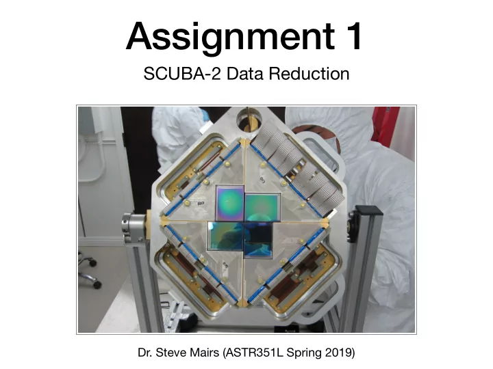
Assignment 1 SCUBA-2 Data Reduction Dr. Steve Mairs (ASTR351L - - PowerPoint PPT Presentation

Assignment 1

SCUBA-2 Data Reduction

• Dr. Steve Mairs (ASTR351L Spring 2019)

Overview

1. Signal vs Noise
 
 2. Data Reduction Methodology
 
 3. Point Spread Function:
 Submillimetre Style
 
 4. Units and Calibration
 
 5. Demonstration

The JCMT is sensitive to molecular clouds with large angular extent 
 and to distant galaxies which appear as point sources

PSF = “Beam” in Radio Astronomy

The beam defines the angular resolution of the image and how 
 much power appears in the “Main beam” in contrast to the “Sidelobes”

First Null
 at 1.2λ/D

PSF = Beam in Radio Astronomy

What the telescope sees is the actual radio brightness distribution in the sky smeared out by (“convolved”) the beam of the telescope. The bigger the beam, the more it smears out, 
 the worse the resolution.

Larger Beam

1 Jy = 1 x 10–26 W m-2 Hz-1 = J s-1 m-2 Hz-1 1 Jy = 1 x 10-23 erg s-1 cm-2 Hz-1

Brightness Unit: The Jansky

Karl Guthe Janksy first discovered 
 radio waves in the Milky Way So we named a unit after him! The amount of energy collected from 
 space by all the radio telescopes ever 
 used to explore the sky would 
 not light a single lightbulb.

Atmosphere is bright and variable 
 at submillimetre wavelengths. Light can be affected 
 by many factors S

• m

e S p a c e t h i n g The JCMT is not 100% reflective, It is also covered with gore-tex!
 
 Pointing and focus uncertainties! The instrumentation has electronic


• noise. Focal planes must be kept 


extremely cold. Temperature 
 fluctuations and power glitches 
 can affect data! *Data Reduction Seeks to 
 Remove All That is Not 
 Real Astronomical Signal

Getting Rid of the Atmosphere

The telescope scans across the sky and across the same region at many different position angles - this is how we can tell what is atmosphere and what is in space! Figures From: 
 Holland et al. 2013 The flux that changes is atmosphere, 
 the flux that stays the same must be stable, 
 astronomical signal

Once we get rid of the signal from the 
 bright and variable atmosphere…
 
 We need to correct for the astronomical
 light that was lost through its journey
 from the top of the
 atmosphere to the telescope!

Data Reduction Seeks to Remove All That is Not Real Astronomical Signal

Extinction Correction 
 Imeasured = I0 exp(-𝛖 x Airmass)
 
 I0 = Imeasured / exp(-𝛖 x Airmass)

𝛖 = Measure of PWV
 (Precipitable Water Vapour)

Weather Grades 1 2 3 4 5

A super-cooled thermometer (0.075 K!) Bolometers (Really Briefly) A small change in temperature = a large change in resistance Light warms up the thermometers, the resistance changes, the current changes! An alternating current = a magnetic field We measure the magnetic field and convert it into a power (in picowatts) Transition Edge Sensors

The Signal in a Single Bolometer

b(t) = f x [e(t) x a(t) + n(t)]

b(t) = Signal Received by a Bolometer f = Scaling Factor (pW -> Jy beam-1) e(t) = Extinction Correction a(t) = Astronomical Signal n(t) = Sources of noise:

• 1. nw = Uncorrelated White noise
• 2. g x nc = Common Mode noise + gain factor
• 3. nf = Excess noise (low freq.)

{

n(t)

An example of Real Time Stream Data From the SCUBA-2 Data Reduction Handbook

• COM: Signal common 


to all bolometers

• FLT: Low frequency 


noise (sky) missed by 
 COM

• AST: Signal, spiking 


as the telescope scans 
 across the source

• RES: Residual white


noise (flat as expected)

SCUBA-2 Data Reduction Overview

• 5 main models applied to the

data which separate sources of noise from astronomical signal

• More than 100 user defined

parameters affect how each model is produced (see Mairs et

• al. 2015. MNRAS 454, 2557 for

examples of DR tests)

• Currently testing 4 different

methods based on the JCMT Gould Belt Survey and the JCMT Legacy Data Release

SCUBA-2 Data Reduction

Chapin et al. 2013, MNRAS. 430, 2545–2573

The Preliminaries

• General cleanup - bad pixels

removed

• Data is flat fielded
• Short duration/high frequency

spikes are removed

• Large “steps” caused by cosmic

rays are removed

• Beginning/end of time series are

smoothed

SCUBA-2 Data Reduction

Chapin et al. 2013, MNRAS. 430, 2545–2573

}

The COM/GAI Models

• The Common Mode (COM) is

similar signal which appears across the majority of the bolometers

• A consequence of variations

in the atmosphere

• The sensitivity of each

bolometer varies from detector to detector

• The GAI model corrects for

the varying sensitivities by comparing a bolometer’s time stream to the common mode

SCUBA-2 Data Reduction

Chapin et al. 2013, MNRAS. 430, 2545–2573

b(t) = f x [e(t) x a(t) + n(t)]

The EXT Model

• EXT refers to the atmospheric

extinction caused by water vapour

• Signalmeas = Signal0 e-𝝊A
• 𝝊 = extinction coefficient (see

Dempsey et al. 2013 MNRAS 430:2534.)

• The JCMT has a water vapour

monitor which is active throughout the observation

SCUBA-2 Data Reduction

Chapin et al. 2013, MNRAS. 430, 2545–2573

b(t) = f x [e(t) x a(t) + n(t)]

The FLT Model

• This model takes the FFT of

the bolometer time series data

• A high pass filter is then

applied to remove the residual 1/f noise after the common mode has been subtracted

• Regridding the map to a

specific pixel size effectively lowpass filters the data below a frequency hat corresponds to the crossing time of a pixel

SCUBA-2 Data Reduction

Chapin et al. 2013, MNRAS. 430, 2545–2573

b(t) = f x [e(t) x a(t) + n(t)]

The AST Model

• AST is the astronomical signal
• The data is gridded onto a map.

The brightness of a given pixel is the weighted average of all the bolometer samples contributing to that pixel. A variance map is also constructed.

• If the SNR of a pixel is above a

specified value, it is included in the AST model

• The AST mode is removed and

saved, leaving a residual map

SCUBA-2 Data Reduction

Chapin et al. 2013, MNRAS. 430, 2545–2573

b(t) = f x [e(t) x a(t) + n(t)]

The NOI Model

• After all of the other noise and

the astronomical signal have been removed, a measurement is made of the residual white noise

• If the white noise converges to

a user-specified tolerance, the final map is produced

• If convergence hasn’t been

achieved, the algorithm begins again at the common mode

SCUBA-2 Data Reduction

Chapin et al. 2013, MNRAS. 430, 2545–2573

b(t) = f x [e(t) x a(t) + n(t)]

SCUBA-2 Calibration: FCFs

Uranus: The Primary Calibrator

The raw data is in units of picowatts (pW) We observe calibrators throughout
 the night, measuring the peak flux and the total flux

http://www.eaobservatory.org/jcmt/instrumentation/continuum/scuba-2/calibration/

Information on our Primary and Secondary calibrators (known fluxes) can be found here: http://www.eaobservatory.org/jcmt/instrumentation/continuum/scuba-2/calibration/calibrators/

By comparing the calibrators’ known
 peak and total flux values to the
 received power, we can measure
 Flux Conversion Factors (FCFs)

SCUBA-2 Calibration: FCFs

http://www.eaobservatory.org/jcmt/instrumentation/continuum/scuba-2/calibration/

Information on our Primary and Secondary calibrators (known fluxes) can be found here: http://www.eaobservatory.org/jcmt/instrumentation/continuum/scuba-2/calibration/calibrators/

*Reduce your calibrator data in the same manner as your observations*

FCFbeam FCFarcsec

pW mJy beam-1 pW mJy arcsec-2 FCFbeam = Speak Ipeak Speak = The known calibrator peak flux Ipeak = The measured peak flux Stotal = The known calibrator total flux Itotal = The measured total flux A = The pixel area in arcsec-2 FCFbeam = Stotal Itotal A

FCF = Flux Conversion Factor

SCUBA-2 Calibration: FCFs

FCF = Flux Conversion Factor

The observatory has measured FCFs over a long period of time to publish nominal values which should work for most observing programs.

FCFbeam FCFarcsec

pW mJy beam-1 pW mJy arcsec-2 The number by which to multiply your map if you wish to measure absolute peak fluxes of discrete sources. http://www.eaobservatory.org/jcmt/instrumentation/continuum/scuba-2/calibration/ The number by which to multiply your map if you wish to use the calibrated map to do aperture photometry. Nominal Values: 450 microns: 491 ± 67 Jy pW-1 beam-1 850 microns: 537 ± 26 Jy pW-1 beam-1 Nominal Values: 450 microns: 4.71 ± 0.50 Jy pW-1 arcsec-2 850 microns: 2.34 ± 0.08 Jy pW-1 arcsec-2 For More Information, See: Dempsey et al. 2013. MNRAS 430:2534 and

The anatomy of a Raw SCUBA-2 File

In “tutorial/”, there are 3 directories: raw/ reduced/ example_reduced/ List the contents of the “raw/” directory:

SCUBA-2 Filename: s8a_20120501_00068_0004.sdf s8a = SCUBA-2, 850 microns, Subarray “a” 20120501 = YYYYMMDD 00068 = Scan Number 0004 = Subscan number (30 seconds of raw power)