Assembly Assembly Computational Challenge: assemble individual short - - PowerPoint PPT Presentation

Assembly

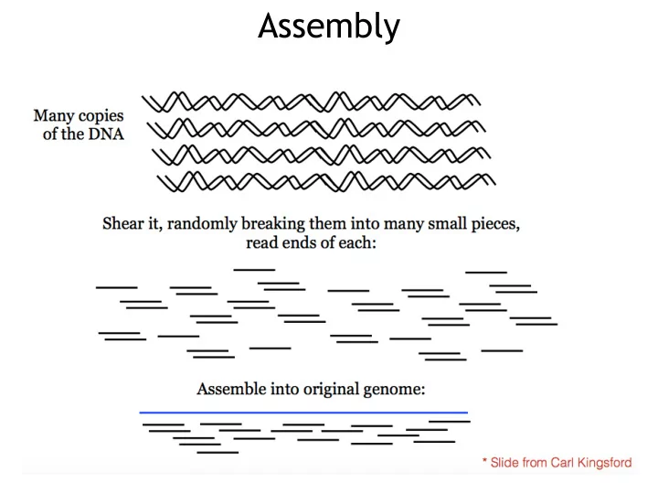
Assembly

Computational Challenge: assemble individual short fragments (reads) into a single genomic sequence (“superstring”)

Problem: Given a set of strings, find a shortest string that contains all of them Input: Strings s1, s2,…., sn Output: A string s that contains all strings s1, s2, …., sn as substrings, such that the length of s is minimized

Shortest common superstring

Shortest common superstring

Overlap Graph

De Bruijn Graph

AT GT CG CA GC TG GG Path visited every EDGE once

Overlap graph vs De Bruijn graph

Some definitions

Eulerian walk/path

zero or

• a. Start with an arbitrary

vertex v and form an arbitrary cycle with unused edges until a dead end is reached. Since the graph is Eulerian this dead end is necessarily the starting point, i.e., vertex v.

Assume all nodes are balanced

• b. If cycle from (a) is not an

Eulerian cycle, it must contain a vertex w, which has untraversed edges. Perform step (a) again, using vertex w as the starting point. Once again, we will end up in the starting vertex w.

• c. Combine the cycles from

(a) and (b) into a single cycle and iterate step (b).

• A vertex v is semibalanced if

| in-degree(v) - out-degree(v)| = 1

• If a graph has an Eulerian path starting from s and

ending at t, then all its vertices are balanced with the possible exception of s and t

• Add an edge between two semibalanced vertices:

now all vertices should be balanced (assuming there was an Eulerian path to begin with). Find the Eulerian cycle, and remove the edge you had added. You now have the Eulerian path you wanted.

Eulerian path

Complexity?

Hidden Markov Models

Markov Model (Finite State Machine with Probs)

Modeling a sequence of weather observations

Hidden Markov Models

Assume the states in the machine are not observed and we can observe some output at certain states.

Hidden Markov Models

Assume the states in the machine are not observed and we can observe some output at certain states.

Hidden: Sunny Hidden: Rainy Observation: Walk Observation: Shop Observation: Clean

s(i-1) s(i+1) s(i)

p(s(i)|s(i − 1)) p(s(i + 1)|s(i))

x(i-1) x(i) x(i+1)

p(x(i − 1)|s(i − 1)) p(x(i)|s(i)) p(x(i + 1)|s(i + 1)) Hidden Observed

Generate a sequence from a HMM

HHHHHHCCCCCCCHHHHHH 3323332111111233332

Hidden: temperature Observed: number of ice creams

Generate a sequence from a HMM

Speech recognition Action recognition

Hidden Markov Models: Applications

Motif Finding

Problem: Find frequent motifs with length L in a sequence dataset Assumption: the motifs are very similar to each other but look very different from the rest part of sequences

ATCGCGCGGCGCGGAATCGDTATCGCGCGCCCAGGTAAGT GCGCGCGCAGGTAAGGTATTATGCGAGACGATGTGCTATT GTAGGCTGATGTGGGGGGAAGGTAAGTCGAGGAGTGCATG CTAGGGAAACCGCGCGCGCGCGATAAGGTGAGTGGGAAAG

Motif: a first approximation

Assumption 1: lengths of motifs are fixed to L Assumption 2: states on different positions on the sequence are independently distributed p(x) =

L

Y

i=1

pi(x(i)) pi(A) = Ni(A) Ni(A) + Ni(T) + Ni(G) + Ni(C)

Motif: (Hidden) Markov models

Assumption 1: lengths of motifs are fixed to L Assumption 2: future letters depend only on the present letter p(x) = p1(x(1))

L

Y

i=2

pi(x(i)|x(i − 1)) pi(A|G) = Ni−1,i(G, A) Ni−1(G)

Motif Finding

Problem: We don’t know the exact locations of motifs in the sequence dataset Assumption: the motifs are very similar to each other but look very different from the rest part of sequences

ATCGCGCGGCGCGGAATCGDTATCGCGCGCCCAGGTAAGT GCGCGCGCAGGTAAGGTATTATGCGAGACGATGTGCTATT GTAGGCTGATGTGGGGGGAAGGTAAGTCGAGGAGTGCATG CTAGGGAAACCGCGCGCGCGCGATAAGGTGAGTGGGAAAG

Hidden state space

null start end

Hidden Markov Model (HMM)

null start end

0.9 0.08 0.95 0.05 0.01 0.99 0.02

How to build HMMs?

Computational problems in HMMs

Hidden Markov Models

Hidden Markov Model

q(i-1) q(i+1) q(i)

• (i-1)
• (i)
• (i+1)

Hidden Observed

Conditional Probability of Observations

Example:

Joint and marginal probabilities

Joint: Marginal:

How to compute the probability of observations

Forward algorithm

Forward algorithm

Forward algorithm

Decoding: finding the most probable states

Similar to the forward algorithm, we can define the following value:

Viterbi algorithm