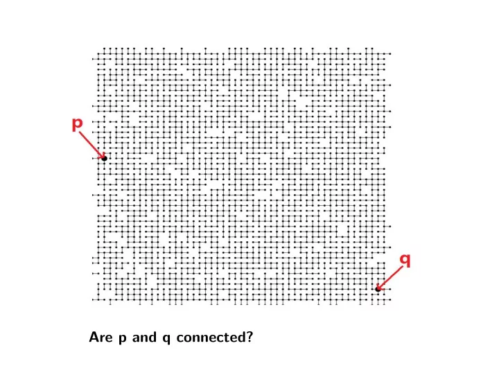
Are p and q connected? Network connectivity Yes, they are - - PowerPoint PPT Presentation

Are p and q connected?

Network connectivity

Yes, they are connected!

Network connectivity

◮ Problem:

Given a set of nodes N and a set of links between pairs of nodes L. Find connectivity for node p and node q.(p∈N,q∈N)

Real World Application

Kruskal

The union-find data structure

Zhengtian Xu Xiaoqing Geng Lihua Qian Ruxuan Zhang Chen Feng

Department of Computer Science and Engineering Shanghai Jiao Tong University

8th December 2016

Outline

Brief Introduction for Union-Find Data Structure Improvement Time Complexity Analysis

Union-Find data structure type

Goal.

Support three operations on a set of elements:

◮ MAKE-SET(x).Create a new set containing only element x. ◮ FIND(x). Return a canonical element in the set containing x. ◮ UNION(x, y). Merge the sets containing x and y.

Union-Find example

6 a 2,7,9,3 b 4,5,8 c

Union-Find example

6 a 2,7,9,3 b 4,5,8 c

FIND(9) = 2

Union-Find example

6 a 2,7,9,3 b 4,5,8 c

FIND(9) = 2 MAKE-SET(1)

Union-Find example

6 a 2,7,9,3 b 4,5,8 c 1 d

FIND(9) = 2 MAKE-SET(1)

Union-Find example

6 a 2,7,9,3 b 4,5,8 c 1 d

FIND(9) = 2 MAKE-SET(1) UNION(2,4)

Union-Find example

6 a 2,7,9,3,4,5,8 e 1 d

FIND(9) = 2 MAKE-SET(1) UNION(2,4)

Union-Find data structure

Representation

Represent each set as a tree of elements.

◮ Each element has a parent pointer in the tree. ◮ The root serves as the canonical element. ◮ FIND(x). Find the root of the tree containing x. ◮ UNION(x, y). Make the root of one tree point to root of

• ther tree.

d a c e b f root parent of e is c

Find operation

Representation

FIND(x). Find the root of the tree containing x. d a c e b g f

Find operation

Representation

FIND(x). Find the root of the tree containing x. d a c e b g f

FIND(g)

Find operation

Representation

FIND(x). Find the root of the tree containing x. d a c e b g f

FIND(g)

Find operation

Representation

FIND(x). Find the root of the tree containing x. d a c e b g f

FIND(g)

Find operation

Representation

FIND(x). Find the root of the tree containing x. d a c e b g f

FIND(g)

Find operation

Representation

FIND(x). Find the root of the tree containing x. d a c e b g f

FIND(g)

Find operation

Representation

FIND(x). Find the root of the tree containing x. d a c e b g f

FIND(g) FIND(d)

Find operation

Representation

FIND(x). Find the root of the tree containing x. d a c e b g f

FIND(g) FIND(d)

Union operation

◮ Maintain an integer rank for each node, initially 0. ◮ Link root of smaller rank to root of larger rank; if tie, increase

rank of new root by 1.

• Note. For now, rank = height.

Union operation

◮ Maintain an integer rank for each node, initially 0. ◮ Link root of smaller rank to root of larger rank; if tie, increase

rank of new root by 1.

union(d, g)

d c i j g k b a h e rank = 2 rank = 1

• Note. For now, rank = height.

Union by rank

◮ Maintain an integer rank for each node, initially 0. ◮ Link root of smaller rank to root of larger rank; if tie, increase

rank of new root by 1.

union(d, g)

d c i j g k b a h e rank = 2

Union by rank

◮ Maintain an integer rank for each node, initially 0. ◮ Link root of smaller rank to root of larger rank; if tie, increase

rank of new root by 1.

union(d, g)

d c l i j g k b a h e rank = 2 rank = 2

Union by rank

◮ Maintain an integer rank for each node, initially 0. ◮ Link root of smaller rank to root of larger rank; if tie, increase

rank of new root by 1.

union(d, g)

d c l i j g k b a h e rank = 3

Union by rank: analysis

Lemma 1. Using union by rank, for every root node r size(r) ≥ 2rank(r) Proof.[ by induction on number of links ]

◮ Base case: singleton tree has size 1 and rank 0. ◮ Inductive hypothesis: assume true after first i links.

Union by rank: analysis

Proof.

◮ Case 1. [ rank(r) > rank(s) ] or [ rank(r) < rank(s) ]

size′(r) ≥ size(r) ≥ 2rank(r) = 2rank′(r) s r size = 8 size = 3 (rank = 2) (rank = 1)

Union by rank: analysis

Proof.

◮ Case 2. [ rank(r) = rank(s) ]

size′(r) = size(r) + size(s) ≥ 2 × size(r) ≥ 2 × 2rank(r) = 2rank(r)+1 = 2rank′(r) s r size = 6 size = 3 (rank = 2) (rank = 1)

Union by rank:analysis

Lemma 2. There are at most

n 2k elements of rank k.

Union by rank:analysis

Lemma 2. There are at most

n 2k elements of rank k.

• Proof. According to Lemma 1, for node has rank k, its sizes are

at least 2k. If the size of all elements is n. Obviously we can get Lemma 2.

Union by rank:analysis

• Theorem. Using Union by rank, any FIND operations takes

O(log2n) time in the worst case, where n is the number of elements; any UNION operations take constant time.

Union by rank:analysis

• Theorem. Using Union by rank, any FIND operations takes

O(log2n) time in the worst case, where n is the number of elements; any UNION operations take constant time. Proof.

◮ The running time of each operation is bounded by the tree

height.

◮ We can know that the height ≤ ⌊log2n⌋

Outline

Brief Introduction for Union-Find Data Structure Improvement Time Complexity Analysis

Improvement

Observation

◮ It is the height of the tree that affects the running time. ◮ When we’re trying to find the root of the tree containing a

given node, we’re touching all the nodes on the path from that node to the root.

So...

◮ Why not make each of those just point to the root? ◮ That’s the idea of path compression!

Path compression

◮ Just after computing the root of the target node, set the

parent of each examined node to point to that root. a b d g i j h e f c height=4 find(j)

Path compression

◮ Just after computing the root of the target node, set the

parent of each examined node to point to that root. a b d g i h e f c j

Path compression

◮ Just after computing the root of the target node, set the

parent of each examined node to point to that root. a b d h e f c j g i

Path compression

◮ Just after computing the root of the target node, set the

parent of each examined node to point to that root. a b e f c j g i d h height=2

Path compression: benefits

◮ The resulting tree is much flatter.

◮ If the target node is very deep, path compression may

dramatically decrease the height of the tree.

◮ Speed up future operations on all the nodes on the path and

• n those referencing them, directly or indirectly.

Path compression: rank vs. height

◮ The rank of a tree does not change during path compression. ◮ ...but the height of a tree may decrease. ◮ Now it is possible that rank = height!

Path compression: rank vs. height

◮ Example: Apply the following operations on the forest below.

◮ Union(a,g) ◮ Find(f) ◮ Find(j)

a b d f e c g h j i 3 2 1 2 1

Path compression: rank vs. height

◮ Union(a,g) ◮ Find(f) ◮ Find(j)

a b d f e c g h j i 3 2 1 2 1

Path compression: rank vs. height

◮ Union(a,g) ◮ Find(f) ◮ Find(j)

a b e d f c g h j i 3 2 1 2 1

Path compression: rank vs. height

◮ Union(a,g) ◮ Find(f) ◮ Find(j)

a b e d f c g i h j 3 2 1 2 1

Path compression: rank vs. height

◮ Union(a,g) ◮ Find(f) ◮ Find(j)

a b e d f c g i h j 3 2 1 2 1 height(a)=2=rank(a)

Outline

Brief Introduction for Union-Find Data Structure Improvement Time Complexity Analysis

Time Complexity Analysis

◮ Without path compression : O(log n) per find instruction. ◮ With path compression : O(log log n) per find instruction.

Time Complexity Analysis

Lemma.

◮ There are at most n 2k nodes with rank k. ◮ rank(parent(x)) > rank(x). ◮ rank(root) ≤ log2 n.

Time Complexity Analysis

Definition.

◮ f (t) = 2 × t

a b rank=2 rank=6 rank(a) > f (rank(b)) happy node, long edge a b rank=2 rank=4 rank(a) ≤ f (rank(b)) sad node, short edge

Time Complexity Analysis

• Observation. In one find operation, at most log log n long edges

are traversed. Proof. r b · · · c d rank ≤ log n rank ≥ 1

• Observation. x is sad for at most rank(x) find operations.

Proof.

◮ rank(parent(x)) > rank(x) ◮ rank(parent(x)) increases per find operation. ◮ After rank(x) find ops,

rank(parent(x)) > rank(x) + rank(x) = f (rank(x))

Time Complexity Analysis

time of all find ops

• find ops #long edges

log log n × m

• find ops #short edges
• e(#find operations when e is short)
• x rank(x)

2n

Time Complexity Analysis

cost of all find operations =

• find ops

(#long edges + #short edges)

• find ops

#long edges ≤ log log n × #find ops

• find ops

#short edges =

• e

(#find operations when e is short) ≤

• x

rank(x) ≤

log n

• k=0

(k × #rank − k − nodes) ≤

∞

• k=0

k × n 2k ≤ 2n

Time Complexity Analysis

• Conclusion. With path compression, time for one find
• p(#find operation ≥ n)is:

O(log log n + 2) = O(log log n) Improvement.

◮ f (t) = 2

t 2 → log ∗n

◮ Ackerman Function → α(n)

Thanks!