Applications James F.W. Purdom, PhD Chair AOMSUC, International - - PowerPoint PPT Presentation

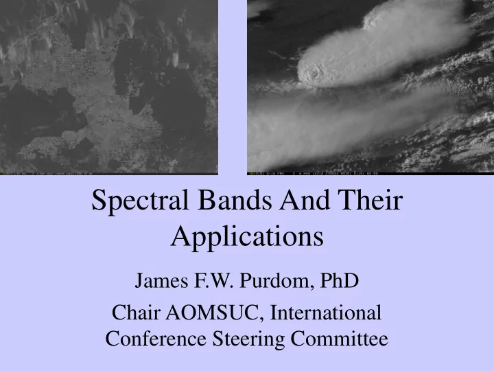
Spectral Bands And Their Applications

James F.W. Purdom, PhD Chair AOMSUC, International Conference Steering Committee

Focus

• Major focus of this presentation is visible, near

infrared and infrared data since those are the types data most NMHSs receive on a routine basis

• Near end there is a short section on microwave

data and products as well as active sensors

– For in depth information concerning the microwave portion of the spectrum and its applications use the resources of the Satellite Virtual Laboratory

Goals

• Understand the difference between visible, near

infrared and infrared radiation (channels) – Understand the influence of surface and atmospheric properties on what we view with a satellite sensor

• Understand the basic underlying principals behind

channel selection and the factors that influence channel selection

• Understand what information can be obtained

using the various satellite channels available from

• perational and research satellites
• Understand how to interpret data from various

channels individually and in combination with

• ther channels

Before we dig into spectral bands

• A brief look into today’s WMO space based
• bserving systems
• A glimpse at the four basic Resolutions

– Spatial – Temporal – Spectral – Radiometric (~Signal to Noise)

• Many of the slides have notes in the notes

section, and there are a number of hidden slides for your inspection at a later time

• There are many (PowerPoint display)

“hidden slides” with different examples

Orbits

• The mainstay orbits for meteorological and

environmental applications

• Sun synchronous Polar orbits
• Geostationary orbits
• Other orbits and specialized applications
• Pro-grade orbits
• Constellations and formation flying

A Brief Reminder: Comparison of geostationary (Geo) and low earth orbiting (Leo) satellite capabilities

Geo Leo

• bserves process itself
• bserves effects of process

(motion and targets of opportunity) repeat coverage in minutes repeat coverage twice daily (t  10 minutes) (t = 12 hours) near full earth disk global coverage best viewing of tropics & mid-latitudes best viewing of poles same viewing angle varying viewing angle differing solar illumination same solar illumination multispectral imager multispectral imager (generally higher resolution) IR only sounder IR and microwave sounder (8 km resolution) (1, 17, 50 km resolution) filter radiometer filter radiometer, interferometer, and grating spectrometer diffraction more than leo diffraction less than geo

Orbit configuration (both Geostationary and Polar)

To learn more about a particular satellite

It’s not quiet that simple

Meteorological Climate Ocean Land Ecological

The spatial and temporal domains of the phenomena being investigated drive the satellite’s observing requirements as a function of space, time, spectra, and signal to noise: and here the trade off begins.

Recall that in satellite remote sensing, four basic parameters need to be addressed: all deal with resolution. The new generation satellites are a giant step forward in all four!!!

– temporal (how often) – spatial (what size) – spectral (what wavelengths and their width) – radiometric (signal-to-noise)

They all must be addressed together in context. Each spatial element has a continuous spectrum that may be used to analyze the surface and atmosphere The spatial and temporal domains of the phenomena being observed drive the satellite systems’ spectral needs as a function of space, time, and signal to noise.

With satellite remote sensing, there are four basic questions that need to be addressed

• They all deal with

resolution:

– temporal (how often) – spatial (what size) – spectral (what wavelengths and their width) – radiometric (signal-to- noise)

Eye Region Hurricane Isabel on 12 September 2003

Temporal (2010 era)

Comparison of animation sequences of severe thunderstorm over western Kansas. Movies at 30, 15, 5 and 1 minute intervals. While 5 minute interval imaging is routine for 2015s, special imaging like this is possible at 1 minute intervals or less.

The spatial and temporal domains of the phenomena being investigated drive the satellite’s observing requirements as a function of space, time, spectra, and signal to noise. These animations are storm overshooting top relative at one minute interval Upper left: 0.5 km visible (500 meters) Lower left: 2 km IR window (2000 meters) Above: IR transparency over visible image

Exploring the limits with 0.5 km imagery @ 6 sec. intervals

The cloud streets moving Northward in the loop appear to be almost rolling, which actually is a reflection of shear across that stably capped cloud street layer (water clouds). Inspection of the two prominent storms as they evolve: the cloud streets can be seen being “tilted” upward into the storm due to increasing vertical motion and buoyancy. For severe storms spatial and temporal synergy!

At least two things to note in this one minute interval 500 meter visible imagers animation

GEO observes the process: A visual representation of the “tilting term” in the vorticity equation

With satellite remote sensing, there are four basic questions that need to be addressed

• They all deal with

resolution:

– temporal (how often)

Vegetation related products which change on slow time frames may be best

• bserved using weekly

data; such as this vegetation and temperature condition index above (derived from AVHRR vegetation index data and thermal infrared data).

Polar product animation

With satellite remote sensing, there are four basic questions that need to be addressed

• They all deal with

resolution:

– temporal (how often) – spatial (what size) – spectral (what wavelengths and their width) – radiometric (signal-to- noise)

GOES and VIIRS Vis (top) 500 vs 375 meters GOES and VIIRS IR (bottom) 2 km vs 375 meters Images taken within 30 seconds of each other, and remapped to same projection

Close up of pervious slide images, Polar view is West of GOES-East satellite

• subpoint. Polar 2 x per day per satellite, GOES as frequently as 1, 2 or10 minutes.

With satellite remote sensing, there are four basic questions that need to be addressed

• They all deal with

resolution:

– temporal (how often) – spatial (what size) – spectral (what wavelengths and their width) – radiometric (signal-to- noise)

Planck blackbody curves (highly non-linear) and IRIS instrument

• bserved

spectrum Planck bb temperature vs wavelength curves very steep at 3.9 microns but relatively flat at 10 microns

Notice the difference in signal to noise at the cold end for 3.9 vs 10.7 (from GOES I/M series)

Illustration of the difference in signal to noise between 10.7 (bottom) and 3.9 (top) micron channels

24

Radiance versus wavelength for blackbodies at 6000 K (sun) and 300 K (earth), notice 3.9 mm region

Today’s satellites measure energy in spectral regions ranging from the visible portion of the electromagnetic spectrum to the far infrared and into the microwave region At visible wavelengths, that energy is only reflected solar radiation; at far infrared wavelengths, that energy is only emitted terrestrial radiation. However for short wavelength infrared channels near 3.9 um energy measured by the satellite can be a mixture of reflected solar and earth emitted radiation during daytime.

Surface and atmospheric properties effect what we view with a satellite sensor (solar left, emitted IR right)

Recall that in satellite remote sensing, four basic parameters need to be addressed: all deal with resolution. The new generation geostationary satellites are a giant step forward in all four!!!

– temporal (how often) – spatial (what size) – spectral (what wavelengths and their width) – radiometric (signal-to-noise)

Each spatial element has a continuous spectrum that may be used to analyze the surface and atmosphere The spatial and temporal domains of the phenomena being observed drive the satellite systems’ spectral needs as a function of space, time, and signal to noise.

Infrared

65,535 ways to “combine” 16 channels

• Single channel 16
• 2 channels per image

120

• 3 channels per image

560

• 4 channels per image

1820

• 5 channels per image

4368

• 6 channels per image

8008

• 7 channels per image

11440

• 8 channels per image

12870

• 9 channels per image

11440

• **********
• 15 channels per image 16
• 16 channels

1

FULL UTILIZATION = BIG CHALLENGE

Spectral Information

• Now let’s look in more detail at the visible,

near infrared and infrared portions of the

• spectrum. Our objective is to get a better

understanding of their unique characteristics and how that information may be used to analyze the land, ocean and atmosphere.

The visible to near infrared portion of the spectrum

Spectral animation of a single AVIRIS scene reveals the power of being able to observe with high spectral

• resolution. Beginning at 400

nanometers ground features are difficult to discern, mainly due to molecular scattering which decreases at longer wavelengths. As we observe the scene at longer wavelengths, some features become distinct (land), while others become

• bscure (apparent decrease in

smoke). Note the effect of the water vapor absorption regions on scene

• brightness. See also next slide.

Spectral animation of a single AVIRIS scene reveals the power of being able to observe with high spectral

• resolution. Beginning at 400

nanometers ground features are difficult to discern, mainly due to molecular scattering which decreases at longer wavelengths. As we observe the scene at longer wavelengths, some features become distinct (land), while others become

• bscure (apparent decrease in

smoke). Note the effect of the water vapor absorption regions on scene brightness.

Smoke - large part. Cloud Hot Area Smoke - small part. Fire Shadow Grass Lake Soil

AVIRIS Spectral Information from the Scene Depicting Cloud, Smoke and Active Burn Areas

4 0 7 0 1 0 1 3 0 1 6 0 1 9 0 2 2 0 2 5

W a v e l e n g t h ( n m )

. 1 1 . 1 .

A p p a re n t R e fle c ta n c e

C l

• u

d F i r e H

• t

A r e a G r a s s L a k e B a r e S

• i

l S m

• k

e ( s m . p a r t . ) S m

• k

e ( l g . p a r t . ) S h a d

• w

AVIRIS Image - Linden CA 20-Aug-1992 224 Spectral Bands: 0.4 - 2.5 mm Pixel: 20m x 20m Scene: 10km x 10km Spectral Signatures of Selected Pixels

Slider: CIRA GeoColor showing smoke and clouds over SE Australia

Slider: CIRA 0.47 micron showing smoke and clouds over SE Australia

Slider: CIRA 0.64 microns showing smoke and clouds over SE Australia

Slider: CIRA 0.86 showing clouds over SE Australia

Slider: CIRA 1.6 microns microns showing clouds over SE Australia

Slider: CIRA 2.3 microns showing fires and clouds over SE Australia

Slider: CIRA Shortwave albedo showing fires and clouds over SE Australia We’ll look at how this product is made from 3.9 and 10.7 micron infrared data a little later. For now the bright spots are fire areas.

Slider: CIRA 0.47 microns showing smoke and clouds over SE Australia

Daytime view of low cloud (water) and a thunderstorm anvil (ice) in different MODIS reflective channels

Now for a look at the reflection from the 1.38 micron MODIS channel in the center of a water vapor absorption region

Let’s look at a few simple examples

• Enhancing single imagery channels
• Using two or three channels to look for a

specific information

54

One advantage of digital data: Image Enhancement: Helping the eye detect Overshooting thunderstorm tops and cloud top temperature

Color bar with warm on left and cold on right

Investigating with Multi-spectral Combinations Being digital and multispectral allows for identification of features by taking advantage of their spectral signatures Given the spectral response

• f a surface or atmospheric feature,

select a part of the spectrum where the reflectance or absorption changes with wavelength If 0.65 μm and 0.85 μm channels see the same reflectance then surface viewed is not vegetation; if 0.85 μm sees considerably higher reflectance than 0.65 μm then surface might be vegetation refl 0.72 μm

0.65 μm 0.85 μm Grass & vegetation

Being digital and multispectral allows for identification of features by taking advantage of their spectral signatures Investigating with Multi-spectral Combinations Given the spectral response

• f a surface or atmospheric feature

Select a part of the spectrum where the reflectance or absorption changes with wavelength e.g. reflection from grass and vegetation refl 0.72 μm

0.65 μm 0.85 μm Grass & vegetation

Animation of vegetation health (stressed to favorable) based on temperature and vegetation index information

Below is a “true color” image from combinations

• r blue, green and red channels

0.646 Red, 0.547 Blue, 0.449 Green “true color”

Below, the same scene viewed with different visible to near infrared wavelength combinations

0.841 Red, 1.225 Blue, 1.600 Green 0.646 Red, 0.547 Blue, 0.449 Green “true color” Non-reflective water bands

Instrument Bands 402-422 nm 433-453 nm 480-500 nm 500-520 nm 545-565 nm 660-680 nm 745-785 nm 845-885 nm Mission Characteristics Sun Synchronous Orbit 705 km Equator Crossing 12:20 PM descending Orbital Period 99 minutes Swath Width 2,801 km Spatial Resolution1.1 km Revisit Time1 day Digitization10 bits Ocean Color: As illustrated by SeaWifs

Ocean color product from MODIS showing the abundance of chlorophyll a across part of the Pacific Ocean.

Daytime multispectral METEOSAT-8 image of large dust storm over Africa. This is made using a combination of images from the 0.6 (Blue), 0.8 (Green) and 1.6 (red) micron

• channels. Click on the image to view animation. Recall 0.6 and 0.8 are used for

vegetation index and 1.6 is used for ice vs water cloud.

Tianjin China: An example of some satellite data analysis capabilities

A single channel animation (3.9 micron channel satellite images) reveals the heat generated by the explosion which

• ccurred at night,

as well as various cloud and land

• features. We’ve

been doing this type activity for decades.

True color image over Bohai Bay, Tianjin, Beijing and North East China

Three channel composite (.74, .86, 1.2) image over Bohai Bay area

Spectral Information

• Now let’s look in more detail at the infrared

portions of the spectrum. Our objective is to get a better understanding of their unique characteristics and how that information may be used to analyze the land, ocean and atmosphere.