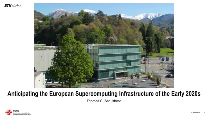
anticipating the european supercomputing infrastructure
play

Anticipating the European Supercomputing Infrastructure of the Early - PowerPoint PPT Presentation

Anticipating the European Supercomputing Infrastructure of the Early 2020s Thomas C. Schulthess T. Schulthess 1 European Commission President Jean-Claude Juncker "Our ambi*on is for Europe to become one of the top 3 world leaders in


  1. Anticipating the European Supercomputing Infrastructure of the Early 2020s Thomas C. Schulthess T. Schulthess � 1

  2. European Commission President Jean-Claude Juncker "Our ambi*on is for Europe to become one of the top 3 world leaders in high-performance compu*ng by 2020" 27 October 2015 European Cloud Initiative (ECI) by the EC [COM(2016) 178, 04/2016] • Help create a digital single market in Europe • Create incentives to share data openly & improve interoperability • Overcome fragmentation (scientific & economic domains, countries, …) • Invest in European HPC ecosystem • Create a dependable environment for data-producers & users to re-use data T. Schulthess � 2

  3. EuroHPC Joint Undertaking (JU): A legal entity for joint procurements between states and the European Commission Members in June 2019 T. Schulthess � 3

  4. Five EuroHPC-JU 
 Petascale systems Installed by 2020 T. Schulthess � 4

  5. Three EuroHPC-JU pre- exascale consortia (TCO ~200-250 mio. each) T. Schulthess � 5

  6. LUMI Consortium • Large consortium with strong national HPC centres and competence provides a unique opportunity for • knowledge transfer; • synergies in operations; and • regionally adaptable user support for extreme-scale systems • National & EU investments (2020-2026) Finland 50 M € Norway 4 M € Poland 5 M € Belgium 15.5 M € Sweden 7 M € Czech Republic 5 M € Switzerland 10 M € Denmark 6 M € EU 104 M € Estonia 2 M € Plus additional investments in applications development T. Schulthess � 6

  7. Strong commitment towards a 
 European HPC ecosystem! T. Schulthess � 7

  8. Kajaani Data Center (LUMI) 2200 m 2 floor space, expandable up to 4600 m 2 100% free cooling @ PUE 1.03 100% hydroelectric energy up to 200 MW One power grid outage in 36 years Extreme connectivity: 
 Kajaani DC is a direct part of the Nordic backbone; 4x100 Gbit/s in place; can be easily scaled up to multi-terabit level Waste heat reuse: effective energy price 35 € /MWh, negative CO2 footprint: 13500 tons reduced every year Zero network downtime since the establishment of the DC in 2012 T. Schulthess � 8

  9. CSCS vision for next generation systems Pursue clear and ambitious goals for successor of Piz Daint • Performance goal: develop a general purpose system (for all domains) with enough performance to run “exascale weather and climate simulations” by 2022, specifically, • Run global model with 1 km horizontal resolution at one simulated year per day throughput on a system with similar footprint at Piz Daint; • Functional goal: converged Cloud and HPC services in one infrastructure • Support most native Cloud services on supercomputer replacing Piz Daint in 2022 • In particular, focus on software defined infrastructure (networking, storage and compute) and service orientation T. Schulthess � 9

  10. Computational power drives spatial resolution 1.E+14 1.E+13 1km 1.E+12 T Co 7999 L180 1.E+11 5km 9km T Co 1999 1.E+10 L160 T Co 1279 16km L137 25km 1.E+09 T L 1279 39km T L 799 T L 511 1.E+08 L91 63km L60 Can the delivery of a 1km-scale T L 319 1.E+07 125km capability be pulled in by a decade? T q 213 L31 208km T q 106 L19 1.E+06 T q 63 L16 1.E+05 1.E+04 1980 1985 1990 1995 2000 2005 2010 2015 2020 2025 2030 2035 Source: Christoph Schär, ETH Zurich, & Nils Wedi, ECMWF T. Schulthess � 10

  11. Leadership in weather and climate European model may be the best – but far away from sufficient accuracy and reliability! Peter Bauer, ECMWF T. Schulthess � 11

  12. Resolving convective clouds (convergence?) Bulk convergence Structural convergence Area-averaged bulk effects upon ambient flow: Statistics of cloud ensemble: E.g., heating and moistening of cloud layer E.g., spacing and size of convective clouds Source: Christoph Schär, ETH Zurich T. Schulthess � 12

  13. Structural and bulk convergence (Panosetti et al. 2018) Statistics of up- & downdrafts Statistics of cloud area 0 0 10 10 8 km 4 km −1 10 2 km −1 10 1 km 500 m −2 10 Factor 4 relative frequency relative frequency −2 10 −3 10 −3 10 grid-scale −4 10 clouds [%] −4 10 −5 10 71 64 54 −5 −6 10 10 47 43 Bulk statistics of updrafts converges No structural convergence −7 −6 10 10 −10 −5 0 5 10 15 −2 0 2 4 10 10 10 10 convective mass flux [kg m −2 s −1 ] cloud area [km 2 ] Source: Christoph Schär, ETH Zurich T. Schulthess � 13

  14. What resolution is needed? • There are threshold scales in the atmosphere and ocean : going from 100 km to 10 km is incremental, 10 km to 1 km is a leap. At 1km • it is no longer necessary to parametrise precipitating convection, ocean eddies, or orographic wave drag and its effect on extratropical storms; • ocean bathymetry, overflows and mixing, as well as regional orographic circulation in the atmosphere become resolved; • the connection between the remaining parametrisation are now on a physical footing. • We spend the last five decades in a paradigm of incremental advances. Here we incrementally improved the resolution of models from 200 to 20km • Exascale allows us to make the leap to 1 km. This fundamentally changes the structure of our models. We move from crude parametric presentations to an explicit, physics based, description of essential processes. • The last such step change was fifty years ago. This was when, in the late 1960s, climate scientists first introduced global climate models, which were distinguished by their ability to explicitly represent extra-tropical storms, ocean gyres and boundary current. Bjorn Stevens, MPI-M T. Schulthess � 14

  15. Our “exascale” goal for 2022 Horizontal resolution 1 km (globally quasi-uniform) Vertical resolution 180 levels (surface to ~100 km) Time resolution Less than 1 minute Coupled Land-surface/ocean/ocean-waves/sea-ice Atmosphere Non-hydrostatic Precision Single (32bit) or mixed precision Compute rate 1 SYPD (simulated year wall-clock day) T. Schulthess � 15

  16. Running COSMO 5.0 & IFS (“the European Model”) at global scale on Piz Daint Scaling to full system size: ~5300 GPU accelerate nodes available Running a near-global (±80º covering 97% of Earths surface) COSMO 5.0 simulation & IFS > Either on the hosts processors: Intel Xeon E5 2690v3 (Haswell 12c). > Or on the GPU accelerator: PCIe version of NVIDIA GP100 (Pascal) GPU T. Schulthess � 16

  17. The baseline for COSMO-global and IFS T. Schulthess � 17

  18. Memory use efficiency Fuhrer et al., Geosci. Model Dev. Discuss., https://doi.org/10.5194/gmd-2017-230, published 2018 0.88 Necessary data transfers Achieved BW MUE = I/O e ffi ciency · BW e ffi ciency = Q B = 0.67 ˆ D B Actual data transfers Max achievable BW 0.76 (STREAM) 600 0.55 w. regard to GPU STREAM (double) a[i] = b[i] (1D) peak BW 500 COPY (double) a[i] = b[i] Memory BW (GB/s) 400 2x lower than peak BW 362 COPY (float) 300 a[i] = b[i] AVG i-stride (float) a[i]=b[i-1]+b[i+1] 200 5-POINT (float) a[i] = b[i] + b[i+1] + b[i-1] + 100 b[i+jstride] +b[i-jstride] 0 0.1 0.1 1 28.2 1000 10 100 1,000 Data size (MB) T. Schulthess � 18

  19. Can the 100x shortfall of a grid-based implementation like COSMO-global be overcome? 600 1. Icosahedral/octahedral grid (ICON/IFS) vs. Lat-long/Cartesian grid (COSMO) GPU STREAM (double) a[i] = b[i] (1D) 500 2x fewer grid-columns COPY (double) 4x a[i] = b[i] Memory BW (GB/s) 400 Time step of 10 ms instead of 5 ms 362 COPY (float) 300 a[i] = b[i] 2. Improving BW efficiency AVG i-stride (float) a[i]=b[i-1]+b[i+1] 200 5-POINT (float) 2x Improve BW efficiency and peak BW a[i] = b[i] + b[i+1] + b[i-1] + 100 b[i+jstride] +b[i-jstride] (results on Volta show this is realistic) 0 0.1 0.1 1 28.2 1000 10 100 1,000 3. Strong scaling Data size (MB) 100 Δ x = 19 km, P100 Δ x = 19 km, Haswell 3x 4x possible in COSMO, but we reduced 
 Δ x = 3.7 km, P100 Δ x = 3.7 km, Haswell available parallelism by factor 1.33 Δ x = 1.9 km, P100 10 Δ x = 930 m, P100 4x 4. Remaining reduction in shortfall SYPD 1 Numerical algorithms (larger time steps) 100x Further improved processors / memory 0.1 But we don’t want to increase the footprint of the 2022 system succeeding “Piz Daint” 0.01 10 100 1000 4888 T. Schulthess � 19 #nodes

  20. What about ensembles and throughput for climate? 
 (Remaining goals beyond 2022) 1. Improve the throughput to 5 SYPD Change the architecture from control flow to data flow centric (reduce necessary data transfers) Necessary data transfers Achieved BW MUE = I/O e ffi ciency · BW e ffi ciency = Q B ˆ D B Actual data transfers Max achievable BW 2. Reduce the footprint of a single simulation by up to factor 10-50 We may have to change the footprint of machines to hyper scale! T. Schulthess � 20

Download Presentation
Download Policy: The content available on the website is offered to you 'AS IS' for your personal information and use only. It cannot be commercialized, licensed, or distributed on other websites without prior consent from the author. To download a presentation, simply click this link. If you encounter any difficulties during the download process, it's possible that the publisher has removed the file from their server.

Recommend


More recommend