Analysis of Solar Observations and Engineering Data from the 2009 - - PowerPoint PPT Presentation

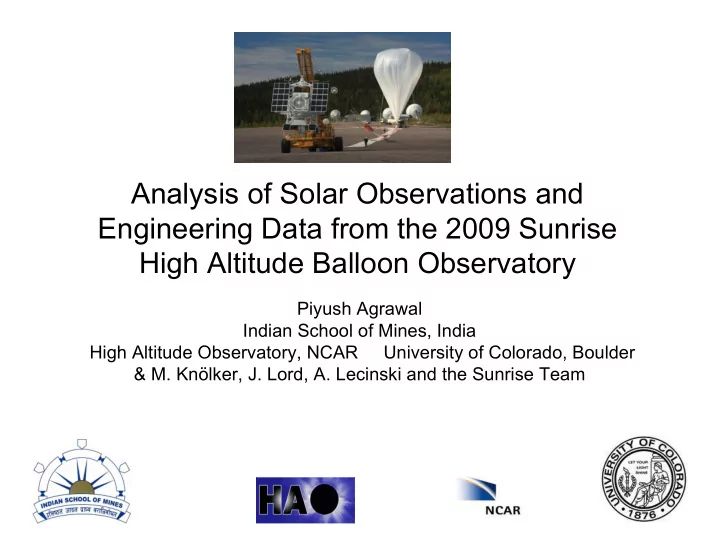
Analysis of Solar Observations and Engineering Data from the 2009 Sunrise High Altitude Balloon Observatory

Piyush Agrawal Indian School of Mines, India High Altitude Observatory, NCAR University of Colorado, Boulder & M. Knölker, J. Lord, A. Lecinski and the Sunrise Team

Sunrise Mission : Key Questions

• What are the origins and properties of the intermittent

magnetic structures?

• How is the magnetic flux brought to and removed from

the solar surface ?

• How does the magnetic field assimilate and provide

energy to heat the upper solar atmosphere ?

• How does the variable magnetic field modify the solar

brightness ?

For this : Sunrise provides Intensity maps at resolution of 0.01 arcsecs in UV

Sunrise Balloon-Borne Solar Observatory

• Gregory telescope, 1-m aperture
• Protective and stabilizing Gondola
• 1.3 kW Solar Array + Li-ion batteries
• Correlating Wavefront Sensor
• Filtergraph : (SuFI)

214nm, 300nm, 313nm, CN, Ca II H

• Magnetograph : (IMaX) Provides

Dopplergrams and Vector Magnetograms in Fe I 525.02 nm

Sunrise Instruments: Fields of View

Telescope FOV = 180 arc sec (approx. 10% of solar diameter)

The REU Project :

• The Solar irradiance variations with the solar

cycle are very small for visible wavelengths i.e. a fraction of a percent, whereas , they are much larger for the UV and EUV . The project aims to relate this variation to the temporal variations in the number density of small bright magnetic structures

Solar UV transmission profile

Different Pointing Sensors:

The 10 Hz Signal

• Sunrise Data Sets are imperfect due to vibrations of

various frequencies. We use a periodic 10 Hertz vibration of varying amplitude as a tracer for good data

• The inherent noise in the sensor was around 2 to 3

ADU (Analog to Digital Unit)

• The level for the 10 Hz range from .1 - 40 ADU
• It appears that the sticking azimuthal drive is one

source of amplification for the 10 Hz …. but its complicated

• Aim : To find the time intervals where the amplitude of

the 10 Hz signal was low

Sticking of the flywheel

10Hz Amplitude and Temperature

d

0 48.6 97.2 136.1 0 48.6 97.2 136.1

d d

Time in minutes Time in minutes

10 hz amplitude

Work Plan I

• The

Engineering Data contains detailed information

• n

pointing characteristics throughout the flight

• Data is in awkward format à develop handling

and extraction tools

• Look at data following A. Lecinski’s sample

analysis

• Use Liss Yaw Pointing Data to sort out
• bserving moments of amplitude within [-

200,200] ADU

• Look for data therein where pointing is locked

• Extraction Tools allow for looking at time

series of variable length à choose appropriate time slice

• Take the FFT of the subset further obtained to

get the amplitude of the 10 Hz vibration

• Analyze Observing Data to check whether

those moments are indeed of better quality

• Proceed with Science Analysis with the Subset
• f Data
• Modify approach if necessary

Continued…..

Time in hours 10 Hz amplitude

10 Hz amplitude distribution

14.00 14.27 14.54 14.81

Good Data Set

17.00 17.14 17.28 17.42 17.54

10 Hz amplitude Bad Data Set

Result I : Liss Yaw plot with varying 10Hz amplitude:

Liss Yaw with low amplitude

• f 10Hz signal

Liss Yaw with high amplitude

Liss Yaw plot for Sorted Data :

Time in hr

Work Plan II

 Determine Contrast of the Images in the 5 SUFI wavelengths  Relate to Solar Irradiance variations in the wavelength range considered

Result II : RMS Intensity Contrast for all wavelengths

Wavelength :

214 nm 300 nm 313 nm 388 nm 397 nm

Average rms intensity contrast vs Wavelength

RMS Intensity Contrast

• f

different patches

• f SuFI 214 nm

Intensity map :

RMS total : 28.19% RMS 1/2 : 27.27 % RMS 1/2 : 29.08 % RMS 1/3 : 27.25 % RMS 1/3 : 30.26 % RMS 1/3 : 25.87 %

RMS INTENSITY CONTRAST

525.02nm 300nm 313nm 388nm 397nm RMS contrast(%) : 16.21 18.76 17.63 15.64 19.30

MAGNETOGRAM

Stokes V Profile

• With the tools developed, we will ‘dig deeper’ to find

the cause of the 10Hz signal

• So far we concentrated on June 9 data, application
• f the analysis tools to the other data will follow
• Then the rms contrast variation with varying

magnetic flux content will be studied using all data suitable

Future work

Acknowledgments:

Michael Knölker Jesse Lord Alice Lecinski Fellow REU students Marty Snow Erin Wood NCAR HAO

Sunrise: Just before the flight

LAUNCH

Data disks O.K. Primary Mirror O.K.

Questions ???

• Thank You