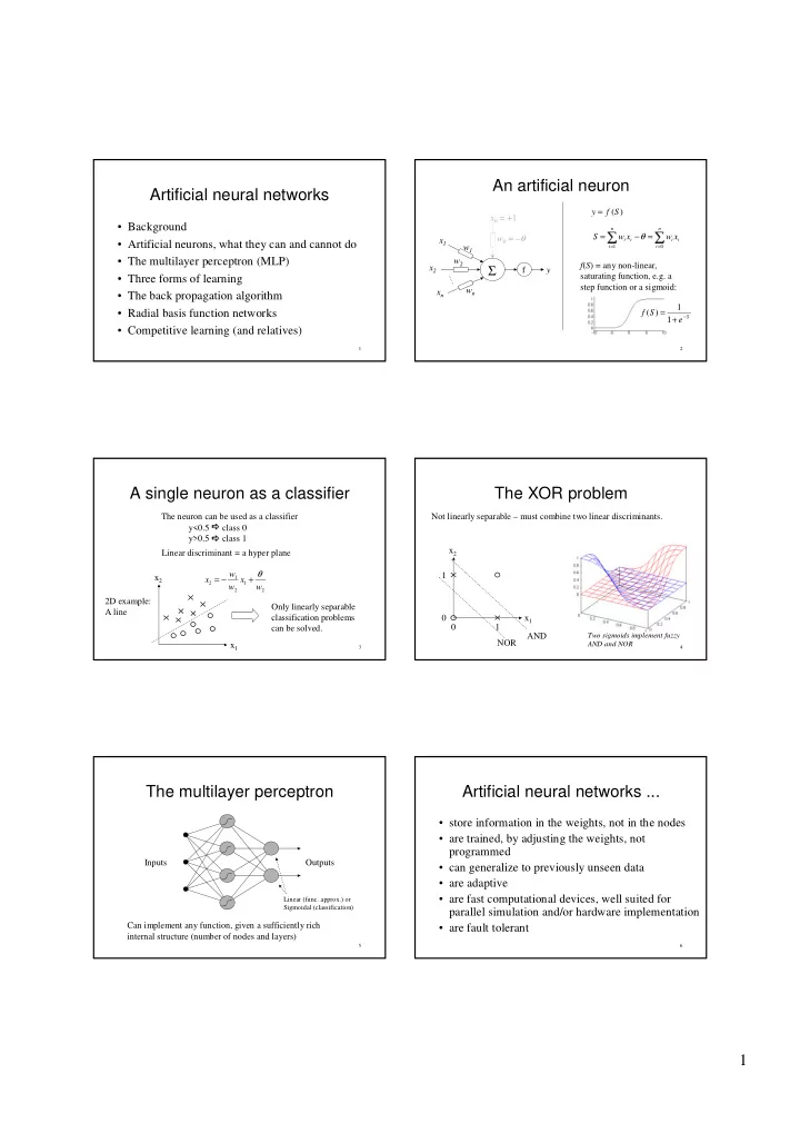
✂ ✂ An�artificial�neuron Artificial�neural�networks y = f ( S ) x 0 =�+1 • Background n n = �✁� − θ = w 0 =�– θ S w x w x x 1 i i i i • Artificial�neurons,�what�they�can�and�cannot�do = = w 1 i 1 i 0 • The�multilayer�perceptron�(MLP) w 2 Σ f ( S )�=�any non-linear,� x 2 f y saturating�function,�e.g.�a� • Three�forms�of�learning step�function�or�a�sigmoid: w n x n • The�back�propagation�algorithm 1 = 1 • Radial�basis�function�networks f ( S ) + − S e • Competitive�learning�(and�relatives) 1 2 A�single�neuron�as�a�classifier The�XOR�problem The�neuron�can�be�used�as�a�classifier Not�linearly�separable�– must�combine�two�linear�discriminants. y<0.5� class�0 y>0.5� class�1 x 2 Linear�discriminant�=�a�hyper plane θ w 1 x 2 = − + 1 x x 2 1 w w 2 2 2D�example: Only�linearly�separable� A�line classification�problems� 0 x 1 0 1 can�be�solved. AND Two�sigmoids�implement�fuzzy� NOR x 1 AND�and�NOR 3 4 The�multilayer�perceptron Artificial�neural�networks�... • store�information�in�the�weights,�not�in�the�nodes • are�trained,�by�adjusting�the�weights,�not� programmed Inputs Outputs • can�generalize�to�previously�unseen�data • are�adaptive • are�fast�computational�devices,�well�suited�for� Linear�(func.�approx.)�or Sigmoidal�(classification) parallel�simulation�and/or�hardware�implementation Can�implement�any�function,�given�a�sufficiently�rich� • are�fault�tolerant internal�structure�(number�of�nodes�and�layers) 5 6 1
✁✂ � ✁ ✆ ✄ ☎ Why�neural�networks? Application�areas (statistical�methods�are�always�at�least�as�good,�right?) Finance Industry • Neural�networks�are statistical�methods • Forecasting • Adaptive�control • Model�independence • Fraud�detection • Signal�analysis • Adaptivity/Flexibility Medicine • Data�mining • Image�analysis • Concurrency Consumer market • Economical�reasons�(rapid�prototyping) • Household�equipment • Character�recognition • Speech�recognition 7 8 Three�forms�of�learning Back�propagation Output�( y ) Unsupervised Supervised Reinforcement Input Desired�output�( d ) Environment Target� Input Error�function function Reward State Action Agent Learning� The�contribution�to�the�error� E – ∂ system E from�a�particular�weight� w ji is� ∂ w ji Error Learning� Action� The�weight�should�be�moved�in� Error�function�and�transfer�function� Suggested� system actions selector proportion�to�that�contribution,�but�in�the� must�both�be�differentiable. other�direction: ∂ E ∆ = − η w ∂ ji w ji 9 10 Back�propagation�update�rule Training�procedure�(1) Network�is�initialised�with�small�random�weights w ji i j k Split�data�in�two�– a� training�set and�a� test�set Assumptions ∂ E ∆ = − η = ηδ w x Error�is�squared�error: ji ∂ j i w ji n The�training�set�is�used�for�training� 1 The�test�set�is�used�to�test�for� = − − 2 ( ) derivative�of�error E d y j j 2 and�is�passed�through�many�times. generalization�(to�see�how� = j 1 − − well�the�net�does�on� y ( 1 y )( d y ) If�node� j is�an�output�node Transfer�(activation)� j j j j δ = Update�weights�after�each� previously�unseen�data). − δ function�is�sigmoid: y ( 1 y ) w Otherwise j j j kj k presentation�( pattern�learning ) k 1 = = or This�is�the�result�the�counts! y f ( S ) − j j + S sum�over�all�nodes�in�the� 1 e j Accumulate�weight�changes�( ∆ w )� derivative�of�sigmoid ’next’�layer�(closer�to�the� until�the�end�of�the�training�set�is� outputs) reached�( epoch or� batch�learning ) 11 12 2
� � � � � Overtraining Network�size E Typical�error�curves • Overtraining�is�more�likely�to�occur�… if�we�train�on�too�little�data Test�or�validation�set�error if�the�network�has�too�many�hidden�nodes if�we�train�for�too�long Training�set�error • The�network�should�be� slightly larger�than�the�size� necessary�to�represent�the�target�function Time�(epochs) • Unfortunately,�the�target�function�is�unknown�... Overtraining • Need�much�more�training�data�than�the�number�of� weights! Cross�validation:�Use�a�third�set,�a� validation�set ,�to�decide�when�to�stop�(find� the�minimum�for�this�set,�and�retrain�for�that�number�of�epochs) 13 14 Training�procedure�(2) Practical�considerations 1. Start�with�a�small�network,�train,�increase�the�size,� • What�happens�if�the�mapping�represented�by�the�data�is�not�a� train�again,�etc.,�until�the�error�on�the� training�set can� function?�For�example,�what�if�the�same�input�does�not�always� be�reduced�to�acceptable�levels. lead�to�the�same�output? • In�what�order�should�data�be�presented?�Sequentially?�At� 2. If�an�acceptable�error�level�was�found,�increase�the� random? size�by�a�few�percent�and�retrain�again,�this�time�using� • How�should�data�be�represented?�Compact?�Distributed? the�cross-validation�procedure�to�decide�when�to�stop.� Publish�the�result�on�the�independent�test�set. • What�can�be�done�about�missing�data? 3. If�the�network�failed�to�reduce�the�error�on�the�training� • Trick�of�the�trade:�Monotonic�functions�are�easier�to�learn�than non-monotonic�functions!�(at�least�for�the�MLP) set,�despite�a�large�number�of�nodes�and�attempts,� something�is�likely�to�be�wrong�with�the�data. 15 16 Radial�basis�functions�(RBF) Geometric�interpretation • Layered�structure,�like�the�MLP,�with�one�hidden�layer • The�input�space�is�covered�with�overlapping�Gaussians. • Output�nodes�are�conventional • Each�hidden�node�… measures�the�distance�between�its�weight�vector�and�the� input�vector�(instead�of�a�weighted�sum) • In�classification,�the�discriminants�become�hyper�spheres� (circles�in�2D). feeds�that�through�a�Gaussian�(instead�of�a�sigmoid) Inputs Outputs 17 18 3
Recommend
More recommend