
SLIDE 1
CS 472 - Perceptron 1
CS 472 - Perceptron 1 Basic Neuron CS 472 - Perceptron 2 - - PowerPoint PPT Presentation
CS 472 - Perceptron 1 Basic Neuron CS 472 - Perceptron 2 Expanded Neuron CS 472 - Perceptron 3 Perceptron Learning Algorithm l First neural network learning model in the 1960s l Simple and limited (single layer models) l Basic concepts
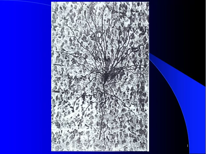
CS 472 - Perceptron 1
CS 472 - Perceptron 2
CS 472 - Perceptron 3
CS 472 - Perceptron 4
CS 472 - Perceptron 5
= = i n i i i n i i
1 1
CS 472 - Perceptron 6
= = i n i i i n i i
1 1
CS 472 - Perceptron 7
= = i n i i i n i i
1 1
CS 472 - Perceptron 8
= = i n i i i n i i
1 1
CS 472 - Perceptron 9
= = i n i i i n i i
1 1
CS 472 - Perceptron 10
l
l
–
–
–
l
l
l
l
l
CS 472 - Perceptron 11
CS 472 - Perceptron 12
CS 472 - Perceptron 13
l
l
l
CS 472 - Perceptron 14
l
l
l
CS 472 - Perceptron 15
l
l
l
CS 472 - Perceptron 16
CS 472 - Perceptron 17
CS 472 - Perceptron 18
CS 472 - Perceptron 19
l
l
l
CS 472 - Perceptron 20
l
l
l
CS 472 - Perceptron 21
l
l
l
CS 472 - Perceptron 22
l
l
l
CS 472 - Perceptron 23
l
l
l
l
CS 472 - Perceptron 24
CS 472 - Perceptron 25
X1 X2
CS 472 - Perceptron 26
X1 X2
CS 472 - Perceptron 27
CS 472 - Perceptron 28
CS 472 - Perceptron 29
CS 472 - Perceptron 30
CS 472 - Perceptron 31
l S|tj – zj| (L1 loss), where j indexes all outputs in the pattern
l Common approach is Squared Error = S(tj – zj)2 (L2 loss)
CS 472 - Perceptron 32
l Since we squared the error on the SSE
CS 472 - Perceptron 33
CS 472 - Perceptron 34
CS 472 - Perceptron 35
CS 472 - Perceptron 36
CS 472 - Perceptron 37
CS 472 - Perceptron 38
ij
CS 472 - Perceptron 39
l
l
l
l
CS 472 - Perceptron 40
CS 472 - Perceptron 41
CS 472 - Perceptron 42
CS 472 - Perceptron 43
CS 472 - Perceptron 44
CS 472 - Perceptron 45
CS 472 - Perceptron 46
CS 472 - Perceptron 47
CS 472 - Perceptron 48
1=1 n
1=1 m
CS 472 - Perceptron 49
CS 472 - Perceptron 50
CS 472 - Perceptron 51
CS 472 - Perceptron 52
l
l
l
l
l
CS 472 - Perceptron 53