Introduction to Neural Networks Jakob Verbeek 2017-2018 Biological - PowerPoint PPT Presentation
Introduction to Neural Networks Jakob Verbeek 2017-2018 Biological motivation Neuron is basic computational unit of the brain about 10^11 neurons in human brain Simplified neuron model as linear threshold unit (McCulloch & Pitts,
Introduction to Neural Networks Jakob Verbeek 2017-2018
Biological motivation Neuron is basic computational unit of the brain about 10^11 neurons in human brain ► Simplified neuron model as linear threshold unit (McCulloch & Pitts, 1943) Firing rate of electrical spikes modeled as continuous output quantity ► Connection strength modeled by multiplicative weight ► Cell activation given by sum of inputs ► Output is non linear function of activation ► Basic component in neural circuits for complex tasks
1957: Rosenblatt's Perceptron Binary classification based on sign of generalized linear function Weight vector w learned using special purpose machines ► Fixed associative units in first layer, sign activation prevents learning ► T ϕ ( x ) w T ϕ( x ) ) sign ( w ϕ i ( x )= sign ( v T x ) Random wiring of associative units 20x20 pixel sensor
Multi-Layer Perceptron (MLP) Instead of using a generalized linear function, learn the features as well Each unit in MLP computes Linear function of features in previous layer ► Followed by scalar non-linearity ► Do not use the “step” non-linear activation function of original perceptron ( 1 ) ) z j = h ( ∑ i x i w ij ( 1 ) x ) z = h ( W ( 2 ) ) y k =σ( ∑ j z j w jk ( 2 ) z ) y =σ( W
Multi-Layer Perceptron (MLP) Linear activation function leads to composition of linear functions Remains a linear model, layers just induce a certain factorization ► Two-layer MLP can uniformly approximate any continuous function on a compact input domain to arbitrary accuracy provided the network has a sufficiently large number of hidden units Holds for many non-linearities, but not for polynomials ►
Feed-forward neural networks MLP Architecture can be generalized More than two layers of computation ► Skip-connections from previous layers ► Feed-forward nets are restricted to directed acyclic graphs of connections Ensures that output can be computed from the input in a single feed- ► forward pass from the input to the output Important issues in practice Designing network architecture ► Nr nodes, layers, non-linearities, etc Learning the network parameters ► Non-convex optimization Sufficient training data ► Data augmentation, synthesis
Activation functions Sigmoid − x ) 1 /( 1 + e Leaky ReLU max (α x, x ) tanh T x ,w 2 T x ) Maxout max ( w 1 ReLU max ( 0, x )
Activation Functions Squashes reals to range [0,1] - Tanh outputs centered at zero: [-1, 1] - Smooth step function - Historically popular since they have - nice interpretation as a saturating “firing rate” of a neuron Sigmoid 1. Saturated neurons “kill” the gradients, need activations to be exactly in right regime to obtain non-constant output 2. exp() is a bit compute expensive Tanh h ( x )= 2 σ( x )− 1 slide from: Fei-Fei Li & Andrej Karpathy & Justin Johnson
Activation Functions Computes f(x) = max(0,x) - Does not saturate (in +region) - Very computationally efficient - Converges much faster than sigmoid/tanh in practice (e.g. 6x) - Most commonly used today ReLU (Rectified Linear Unit) [Nair & Hinton, 2010] slide from: Fei-Fei Li & Andrej Karpathy & Justin Johnson
Activation Functions - Does not saturate: will not “die” - Computationally efficient - Converges much faster than sigmoid/tanh in practice! (e.g. 6x) Leaky ReLU [Mass et al., 2013] [He et al., 2015] slide from: Fei-Fei Li & Andrej Karpathy & Justin Johnson
Activation Functions • Does not saturate: will not “die” • Computationally efficient - Maxout networks can implement ReLU networks and vice-versa - More parameters per node Maxout T x ,w 2 T x ) max ( w 1 [Goodfellow et al., 2013]
Training feed-forward neural network Non-convex optimization problem in general Typically number of weights is very large (millions in vision applications) ► Seems that many different local minima exist with similar quality ► 1 N N ∑ i = 1 L ( f ( x i ) , y i ;W )+λ Ω( W ) Regularization L2 regularization: sum of squares of weights ► “Drop-out”: deactivate random subset of weights in each iteration ► Similar to using many networks with less weights (shared among them) Training using simple gradient descend techniques Stochastic gradient descend for large datasets (large N) ► Estimate gradient of loss terms by averaging over a relatively small ► number of samples
Training the network: forward propagation Forward propagation from input nodes to output nodes Accumulate inputs via weighted sum into activation ► Apply non-linear activation function f to compute output ► Use Pre(j) to denote all nodes feeding into j a j = ∑ i ∈ Pre ( j ) w ij x i x j = f ( a j )
Training the network: backward propagation Node activation and output a j = ∑ i ∈ Pre ( j ) w ij x i x j = f ( a j ) Partial derivative of loss w.r.t. activation g j = ∂ L ∂ a j x i Partial derivative w.r.t. learnable weights w ij ∂ a j ∂ L = ∂ L = g j x i ∂ w ij ∂ a j ∂ w ij Gradient of weight matrix between two layers given by outer-product of x and g
Training the network: backward propagation Back-propagation layer-by-layer of gradient from loss to internal nodes Application of chain-rule of derivatives ► a j = ∑ i ∈ Pre ( j ) w ij x i Accumulate gradients from downstream nodes x j = f ( a j ) Post(i) denotes all nodes that i feeds into ► Weights propagate gradient back ► g i = ∂ L ∂ a i Multiply with derivative of local activation function ∂ a j ∂ L ∂ L = ∑ j ∈ Post ( i ) ∂ x i ∂ a j ∂ x i = ∑ j ∈ Post ( i ) g j w ij g i =∂ x i ∂ L ∂ a i ∂ x i = f ' ( a i ) ∑ j ∈ Post ( i ) w ij g j
Training the network: forward and backward propagation Special case for Rectified Linear Unit (ReLU) activations f ( a )= max ( 0, a ) Sub-gradient is step function 0 if a ≤ 0 f ' ( a )= { 1 otherwise Sum gradients from downstream nodes 0 if a i ≤ 0 g i = { ∑ j ∈ Post ( i ) w ij g j otherwise Set to zero if in ReLU zero-regime ► Compute sum only for active units ► Gradient on incoming weights is “killed” by inactive units Generates tendency for those units to remain inactive ► ∂ a j ∂ L = ∂ L = g j x i ∂ w ij ∂ a j ∂ w ij
Convolutional Neural Networks How to represent the image at the network input? Input example : an image Output example: class label airplane dog automobile frog bird horse cat ship deer truck
Convolutional neural networks A convolutional neural network is a feedforward network where Hidden units are organizes into images or “response maps” ► Linear mapping from layer to layer is replaced by convolution ►
Convolutional neural networks Local connections: motivation from findings in early vision Simple cells detect local features ► Complex cells pool simple cells in retinotopic region ► Convolutions: motivated by translation invariance Same processing should be useful in different image regions ►
Preview: ConvNet is a sequence of Convolution Layers, interspersed with activation functions 32 28 CONV, ReLU e.g. 6 5x5x3 32 28 filters 3 6 slide from: Fei-Fei Li & Andrej Karpathy & Justin Johnson Fei-Fei Li & Andrej Karpathy & Justin Johnson Lecture 7 - 27 Jan 2016
Preview: ConvNet is a sequence of Convolutional Layers, interspersed with activation functions 32 28 24 …. CONV, CONV, CONV, ReLU ReLU ReLU e.g. 6 e.g. 10 5x5x 6 5x5x3 filters 32 28 24 filters 3 6 10 slide from: Fei-Fei Li & Andrej Karpathy & Justin Johnson
The convolution operation
The convolutjon operatjon
Local connectivity Locally connected layer without weight sharing Convolutjonal layer used in CNN Fully connected layer as used in MLP
Convolutional neural networks Hidden units form another “image” or “response map” Followed by point-wise non-linearity as in MLP ► Both input and output of the convolution can have multiple channels E.g. three channels for an RGB input image ► Sharing of weights across spatial positions decouples the number of parameters from input and representation size Enables training of models for large input images ►
Convolution Layer 32x32x3 image height 32 width 32 depth 3 slide from: Fei-Fei Li & Andrej Karpathy & Justin Johnson
Convolution Layer 32x32x3 image 5x5x3 filter 32 Convolve the filter with the image i.e. “slide over the image spatially, computing dot products” 32 3 slide from: Fei-Fei Li & Andrej Karpathy & Justin Johnson
Convolution Layer Filters always extend the full 32x32x3 image depth of the input volume 5x5x3 filter 32 Convolve the filter with the image i.e. “slide over the image spatially, computing dot products” 32 3 slide from: Fei-Fei Li & Andrej Karpathy & Justin Johnson
Convolution Layer 32x32x3 image 5x5x3 filter 32 1 hidden unit: dot product between 5x5x3=75 input patch and weight vector + bias T x + b w 32 3 slide from: Fei-Fei Li & Andrej Karpathy & Justin Johnson
Recommend
More recommend
Explore More Topics
Stay informed with curated content and fresh updates.
