
SLIDE 1
-
Allman & Kaas, 1981 Zeki, - - PowerPoint PPT Presentation
Allman & Kaas, 1981 Zeki, 1978 IT neurons are tolerant to identity-preserving transformations Position Scale Context Rust & DiCarlo, 2012 Selectivity and invariance
Allman & Kaas, 1981 Zeki, 1978
Position Scale Context
IT neurons are tolerant to identity-preserving transformations
Rust & DiCarlo, 2012
The geometry of selectivity and invariance. The three axes are three image dimensions (e.g., the values of three pixels in an image). Real images require several thousand dimensions, but we use three for simple visualization. Any point in the space corresponds to a different image. The gray surface represents a continuous subset, or manifold, of images of a particular object. If a hypothetical neural population effectively encodes this object's identity, all object images from this manifold will yield patterns of neural responses that are distinguishable from the patterns of responses induced by other sets of images. Moving along the surface of the manifold changes the image itself but maintains the ability of the neural population to discriminate the image from others. This is a direction of invariance. Moving away from, or orthogonal to, the surface of the manifold changes the image in a way that prevents the population from effectively discriminating. This is a direction of selectivity. The manifold shown here corresponds to a set of population responses that are selective for proboscis monkeys, not just for image patches with similar color and texture, but are also invariant to changes in size (near vs far) and context (face only vs face and body).
Selectivity and invariance
Freeman & Ziemba, 2011
Object tangling
DiCarlo & Cox, 2007
Untangling object manifolds along the ventral visual stream
DiCarlo & Cox, 2007
The form processing pathway maintains an “equally distributed” representation of images
3410 Neurobiology: Sheinberg and Logothetis
Correlation of IT activity and perceptual state during binocular rivalry (Sheinberg and Logothetis, 1997)
V1 V2 V4 20 40 60 80 100 Excited when stimulus suppressed Excited when stimulus perceived Frequency (%) MT (V5) TPO, TEm, TEa
Correlation of IT activity and perceptual state during binocular rivalry (Logothetis, 1998)
Ungerleider & Mishkin, 1982
Ventral pathway Form, recognition, memory Dorsal pathway Space, motion, action
Why motion?
George Mather, Patrick Cavanagh, and others
Figure 1 First demonstration of direction selectivity in macaque MT/V5 by Dubner & Zeki (1971). (a) Neuronal responses to a bar of light swept across the receptive field in different directions (modified from figure 1
direction indicated by the arrow. The neuron’s preferred direction was up and to the right. (b) Oblique penetration through MT (modified from figure 3 of Dubner & Zeki 1971) showing the shifts in preferred direction indicative of the direction columns subsequently demonstrated by Albright et al. (1984). See also Figure 4.
Maunsell & V an Essen, 1983
MT
Hubel & Wiesel, 1968
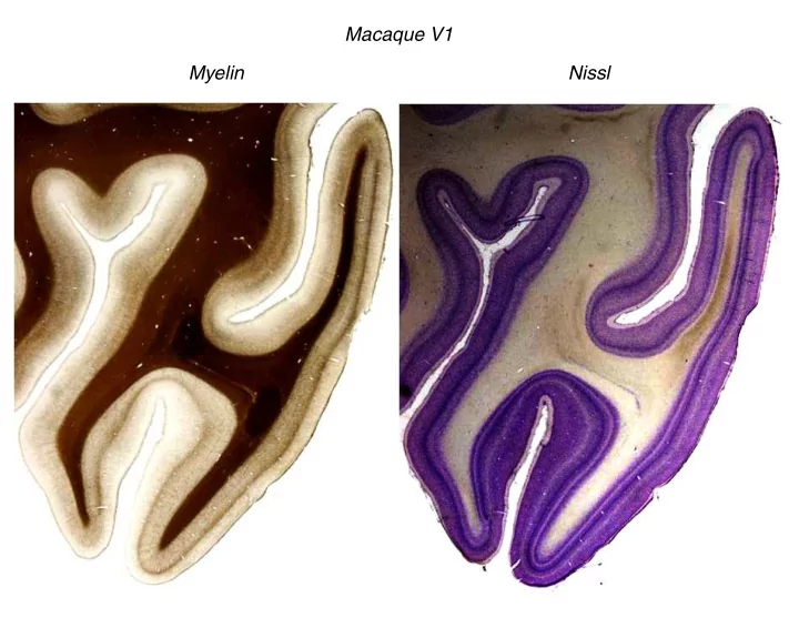
V1
Movshon & Newsome, 1996
Movshon & Newsome, 1996
Figure 6 Center-surround interactions in MT. (A) Effect of contrast on center-surround interactions for one MT
same test using a low-contrast dot pattern (0.7 cd/m2) revealed strong area summation with increasing
high and low contrast. Surround suppression was quantified as the percent reduction in response between the largest dot patch (35◦ diameter) and the stimulus eliciting the maximal response. Each dot represents data from one neuron; the dashed diagonal is the locus of points for which the surround suppression was unchanged by contrast. The circled dot is the cell from panel A. (C) Asymmetries in the spatial
are potentially useful for calculating spatial changes in flow fields that may be involved in the computation of structure from motion. Neurons whose receptive fields have circularly symmetric surrounds (top) are postulated to underlie figure-ground segregation. The first- (middle) and second-order (bottom) directional derivatives can be used to determine surface tilt (or slant) and surface curvature, respectively (Buracas & Albright 1996). Panels A and B are from Pack et al. 2005. Center-surround interactions in MT
1136
AND
ESSEN
100 75 AVERAGE RATE OF 50 FIRING
(
i mpulses /
I- S) 25-
VT / / +
I 0 J?
11-1111111111111111-llllllllllllllllllll 05 . 2 8 32 128 512 SPEED (deg/s 1
1. .* A . . *- A. Il... . . . rL. I I I I I I05 . 1 A a+
lk
L h UUICL J-d-- 2 4 8 16 32 64 128 256 512
Responses
unit in MT to stimuli moving in its preferred direction at different speeds. In this and all subsequent plots the speed axis is logarithmic. Bars indicate the standard errors
for five repetitions
A dashed line marks the background rate
This unit, like most in MT, had a sharp peak in its response curve. Summed response histograms in the lower half of the figure show that the peak rate
closely follows the average rate
Tic marks under each histogram denote times
The receptive field was 15” across and each stimulus traversed 20”.
stimulus repetitions to achieve a satisfactory standard error of the mean. Responses from four units that showed narrow tuning for stimulus speed are illus- trated in Fig. 6A. The abscissa is again log- arithmic. All these units showed inhibition to speeds that were far from their preferred speed, and portions of the tuning curves that are below background rate firing are indi- cated by dashed lines. In the overall popu- lation, a few units had responses that re- mained high toward one end of the range or the other, but the great majority had a clear
at speeds far from the op- timum was seen only occasionally
slow side of the peak but was more common
relation between the sharpness of tuning for speed and that for direction in our sample. Many units were examined with manual monocular stimulation for evidence of dif- ferent preferred monocular
preferred direction, the monocular preferred speeds were similar to one another and to the binocular value. Orban et al. (41) reported that neurons in cat areas 17 and 18 could be grouped into four distinct classes based on the speeds to
Speed tuning
Movshon, Adelson, Gizzi & Newsome, 1985
Movshon, Adelson, Gizzi & Newsome, 1985
Gratings, plaids, and coherent motion
Movshon, Adelson, Gizzi & Newsome, 1985
Grating response Predicted plaid response
Grating responses Plaid responses V1 cell
90o
MT component cell
90o
MT pattern cell
135o Movshon, Adelson, Gizzi & Newsome, 1985
Movshon & Newsome, 1996
Khawaja, Tsui & Pack, 2009
MST also contains a high proportion of pattern cells
Khawaja, Tsui & Pack, 2009
Local field potentials may reveal stages in pattern computation
Khawaja, Tsui & Pack, 2009
Local field potentials may reveal stages in pattern computation
Movshon, Adelson, Gizzi & Newsome, 1985
Grating responses Plaid responses MT pattern cell Components of the optimal plaid Plaids containing the optimal grating
Movshon et al, 1985 Hubel & Wiesel, 1962
Simple cortical cell Lateral geniculate cells
ωt ωx ωy ωt ωx ωy
Simoncelli & Heeger., 1998
Linear
Gain control Output nonlinearity Linear
Gain control Output nonlinearity
ωt ωx ωy
Simoncelli & Heeger., 1998
1D motion stimuli
Majaj, Carandini & Movshon, 2007
Majaj, Carandini & Movshon, 2007
Majaj, Carandini & Movshon, 2007
0.5 1.0 50 0.5 1.0 50 0.5 1.0 50 0.5 1.0 50 Time (s)
549l009
Global preferred Local preferred Global preferred Local null Global null Local preferred Global null Local null
Firing rate (imp/s)
Hedges, Gartshteyn, Kohn, Rust, Shadlen, Newsome & Movshon, 2011
0.5 1.0 50 0.5 1.0 50 0.5 1.0 50 0.5 1.0 50 Time (s)
549l009
Global preferred Local preferred Global preferred Local null Global null Local preferred Global null Local null
Firing rate (imp/s)
Hedges, Gartshteyn, Kohn, Rust, Shadlen, Newsome & Movshon, 2011
0.5 1.0 50 0.5 1.0 50 0.5 1.0 50 0.5 1.0 50 Time (s)
549l009
Global preferred Local preferred Global preferred Local null Global null Local preferred Global null Local null
Firing rate (imp/s)
Hedges, Gartshteyn, Kohn, Rust, Shadlen, Newsome & Movshon, 2011
0.5 1.0 50 0.5 1.0 50 0.5 1.0 50 0.5 1.0 50 Time (s)
549l009
Firing rate (imp/s)
50 50 50 50 50 50 50 3 50 3 3 3 10 20 40 80 160 320 640 Time (s)
Firing rate (ips) Temporal offset (ms)
Global preferred Local preferred Global preferred Local null Global null Local preferred Global null Local null 210 105 52.5 26.3 13.1 6.6 3.3 ∞
Global speed (deg/s)
Hedges et al, 2011
n = 101
0.0 0.5 1.0 1.5 Local dominance 0.00 0.05 0.10 0.15 Proportion of cells Purely global Purely local How do local and global motion signals interact?
Hedges, Gartshteyn, Kohn, Rust, Shadlen, Newsome & Movshon, 2011
Linear
Gain control Output nonlinearity Linear
Gain control Output nonlinearity
ωt ωx ωy
Simoncelli & Heeger, 1998; Rust, Mante, Simoncelli & Movshon, 2006
Rust, Mante, Simoncelli & Movshon, 2006
Rust, Mante, Simoncelli & Movshon, 2006
Rust, Mante, Simoncelli & Movshon, 2006
ωt ωx ωy ωt ωx ωy ωt ωx ωy
MT receptive field
Nishimoto & Gallant, 2011
Nishimoto & Gallant, 2011
Nishimoto & Gallant, 2011
Nishimoto & Gallant, 2011
Nishimoto & Gallant, 2011
ωt ωx ωy ωt ωx ωy ωt ωx ωy
Nishimoto & Gallant, 2011
Ned Block
Opinion
TRENDS in Cognitive Sciences Vol.9 No.2 February 2005
V1 (striate cortex) V2 V3 V4 V5 (MT) V5A V3A Activation
Local and global motion signals