Alan Guth, Dynamics of Homogeneous Expansion, Part IV, 8.286 Lecture - - PowerPoint PPT Presentation

alan guth dynamics of homogeneous expansion part iv 8 286
SMART_READER_LITE
LIVE PREVIEW

Alan Guth, Dynamics of Homogeneous Expansion, Part IV, 8.286 Lecture - - PowerPoint PPT Presentation

Alan Guth, Dynamics of Homogeneous Expansion, Part IV, 8.286 Lecture 8, October 1, 2013, p. 1. 8.286 Leture 8 Summary: Mathematial Model Otober 1, 2013 t i time of initial picture DYNAMICS OF R max ,i initial maximum radius


slide-1
SLIDE 1

Alan Guth, Dynamics of Homogeneous Expansion, Part IV, 8.286 Lecture 8, October 1, 2013, p. 1.

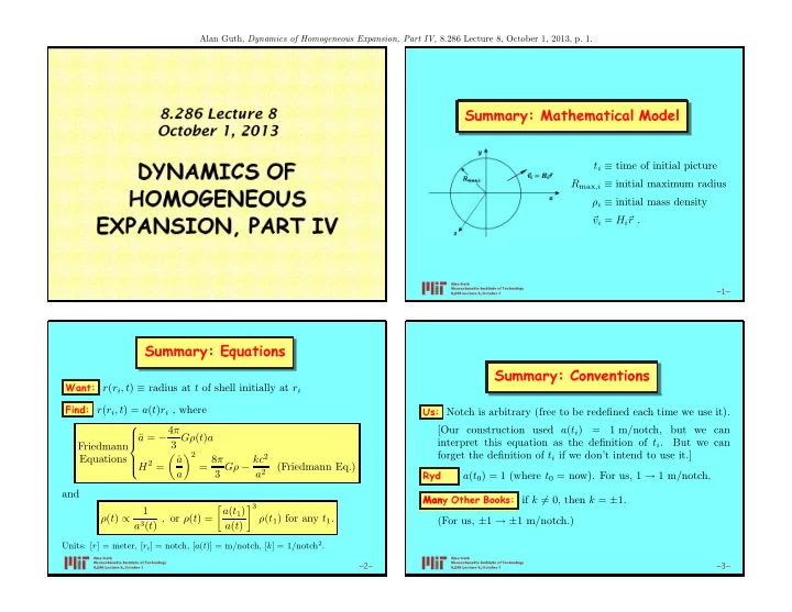
8.286 Le ture 8 O tober 1, 2013 DYNAMICS OF HOMOGENEOUS EXPANSION, PART IV Summary: Mathemati al Model

ti ≡ time of initial picture Rmax,i ≡ initial maximum radius ρi ≡ initial mass density

  • vi = Hi

r .

Alan Guth Massa husetts Institute
  • f
T e hnology 8.286 Le ture 8, O tober 1

–1–

Summary: Equations Want: r(ri, t) ≡ radius at t of shell initially at ri

r(ri, t) = a(t)ri , where

Find:

   4π ¨ a = Gρ(t)a Friedmann  Equations   −  3 H2 = ˙ a a 2 8π kc2 = Gρ 3 − (Friedmann Eq.) a2 and ρ 1 a(t ) ( ) =

1

t) ∝ , or ρ(t ρ(t a3(t) a(t)

1) for any t1.

  • 3

Units: [r] = meter, [ri] = notch, [a(t)] = m/notch, [k] = 1/notch2.

Alan Guth Massa husetts Institute
  • f
T e hnology 8.286 Le ture 8, O tober 1

–2–

Summary: Conventions Us: Notch is arbitrary (free to be redefined each time we use it).

Our construction used a(ti) = 1 m/notch, but we can nterpret this equation as the definition of ti. But we can

  • rget the definition of ti if we don’t intend to use it.]
en: a(t0) = 1 (where t0 = now). For us, 1 → 1 m/notch. y Other Books: if k = 0, then k = ±1.

For us, ±1 → ±1 m/notch.) [ i f

Ryd Man
  • (
Alan Guth Massa husetts Institute
  • f
T e hnology 8.286 Le ture 8, O tober 1

–3–

Many Other Books:
slide-2
SLIDE 2

Alan Guth, Dynamics of Homogeneous Expansion, Part IV, 8.286 Lecture 8, October 1, 2013, p. 2.

Summary: Types
  • f
Solutions

8 ˙ a2 πG ρ(t =

1)a3(t1)

3 a(t) − kc2 . For intuition, remember that k ∝ −E, where E is a measure of the energy of the system.

Types
  • f
Solutions:

1) k < 0 (E > 0): unbound system. ˙ a2 > (−kc2) > 0, so the universe expands

  • forever. Open Universe.

2) k > 0 (E < 0): bound system. ˙ a2 = ≥ ⇒ 8πG ρ(t amax =

1)a3(t1) .

3 kc2 Universe reaches maximum size and then contracts to a Big Crunch. Closed Universe. –4–

3) k = 0 (E = 0): critical mass de

2

8πG kc2 H = ρ 3 − = a2

=0

Flat Universe.

  • Summary: ρ > ρc ⇐

⇒ closed, ρ < ρc ⇐ ⇒ open, ρ = ρc ⇐ ⇒ flat. Numerical value: For H = 67.3 km-s−1-Mpc−1 (Planck 2013 plus

  • ther experiments),

ρc = 8.4 × 10⁻³⁰ g/cm3 ≈ 5 proton masses per m3. ρ Definition: Ω ≡ . ρc nsity. ⇒ 3H2 ρ ≡ ρc = 8πG .

Alan Guth Massa husetts Institute
  • f
T e hnology 8.286 Le ture 8, O tober 1

–5–

Summary: Evolution
  • f
a Flat Universe

If k = 0, then ˙ a2 8πG const da const = ρ = = = a 3 a3 ⇒ dt a1/2 2 = ⇒ a1/2a da = const dt = ⇒ a3/2 = (const)t + c′ . 3 Choose the zero of time to make c′ = 0, and then a(t) t2/3 . ∝

Alan Guth Massa husetts Institute
  • f
T e hnology 8.286 Le ture 8, O tober 1

–6–

slide-3
SLIDE 3

MIT OpenCourseWare http://ocw.mit.edu

8.286 The Early Universe

Fall 2013 For information about citing these materials or our Terms of Use, visit: http://ocw.mit.edu/terms.