
SLIDE 1
98
Explicit Density p(x)
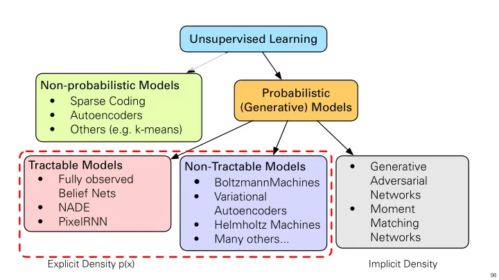
Unsupervised Learning Non-probabilistic Models
- Sparse Coding
- Autoencoders
- Others (e.g. k-means)
Probabilistic (Generative) Models Tractable Models
- Fully observed
Belief Nets
- NADE
- PixelRNN
Non-Tractable Models
- BoltzmannMachines
- Variational
Autoencoders
- Helmholtz Machines
- Many others...
Implicit Density
- Generative
Adversarial Networks
- Moment
Matching Networks