Acquiring Images Brian Curless University of Washington The - - PDF document

acquiring images
SMART_READER_LITE
LIVE PREVIEW

Acquiring Images Brian Curless University of Washington The - - PDF document

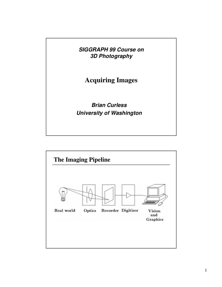
SIGGRAPH 99 Course on 3D Photography Acquiring Images Brian Curless University of Washington The Imaging Pipeline 1 Overview Pinhole camera Lenses Principles of operation Limitations Charge-coupled devices Principles of


slide-1
SLIDE 1

1

Acquiring Images

Brian Curless University of Washington SIGGRAPH 99 Course on 3D Photography

The Imaging Pipeline

slide-2
SLIDE 2

2

Overview

Pinhole camera Lenses

  • Principles of operation
  • Limitations

Charge-coupled devices

  • Principles of operation
  • Limitations

The pinhole camera

The first camera - “camera obscura” - known to Aristotle. Small aperture = high fidelity but requires long exposure or bright illumination

slide-3
SLIDE 3

3

Pinhole camera

If aperture is too small, then diffraction causes blur.

[Figure from Hecht87]

Lenses

Lenses focus a bundle of rays to one point. => can have larger aperture.

[Figure from Hecht87]

slide-4
SLIDE 4

4

Lenses

A lens images a bundle of parallel rays to a focal point at a distance, f, beyond the plane of the lens. Note: f is a function of the index of refraction of the lens. An aperture of diameter, D, restricts the extent of the bundle of refracted rays.

Lenses

For economical manufacture, lens surfaces are usually spherical. A spherical lens is behaves ideally if is small: φ φ φ φ φ ≈ − + − = ... ! 5 ! 3 sin

5 3

The angle restriction means we consider rays near the optical axis -- “paraxial rays.”

slide-5
SLIDE 5

5

Lenses

For a “thin” lens, we ignore lens thickness, and the paraxial approximation leads to the familiar Gaussian lens formula:

f d d

i

  • 1

1 1 = +

  • d

i

d f

[Figure from Hecht87]

Cardinal points of a lens system

Most cameras do not consist of a single thin lens. Rather, they contain multiple lenses, some thick. A system of lenses can be treated as a “black box” characterized by its cardinal points.

slide-6
SLIDE 6

6

Focal and principal points

The focal and principal points and the principal “planes” describe the paths of rays parallel to the

  • ptical axis.

Nodal points

The nodal points describe the paths of rays that are not refracted, but are translated down the

  • ptical axis.
slide-7
SLIDE 7

7

Cardinal points of a lens system

If:

  • the optical system is surrounded by air
  • and the principal planes are assumed planar

then

  • the nodal and principal points are the same

The system still obeys Gauss’s law, but all distances are now relative to the principal points.

Depth of field

Lens systems do have some limitations. First, points that are not in the object plane will appear out of focus. The depth of field is a measure of how far from the

  • bject plane points can be before appearing “too

blurry.”

slide-8
SLIDE 8

8

Monochromatic aberrations

Allowing for the next higher terms in the sin approximation:

! 3 ... ! 5 ! 3 sin

3 5 3

φ φ φ φ φ φ − ≈ − + − =

…we arrive at the third order theory. Deviations from ideal optics are called the primary or Seidel aberrations:

  • Spherical aberration
  • Coma
  • Astigmatism
  • Petzval curvature
  • Distortion

Distortion

Cause: Oblique rays bent by the edges of the lens Effect: Non-radial lines curve out (barrel) or curve in (pin cushion) Ways of improving: Symmetrical design.

[Figure from Hecht87]

slide-9
SLIDE 9

9

Distortion

[Figures from Hecht87]

Chromatic aberration

Cause: Index of refraction varies with wavelength. Effect: Focus shifts with color, colored fringes on highlights Ways of improving: Achromatic designs

[Figure from Hecht87]

slide-10
SLIDE 10

10

Flare

Light rays refract and reflect at the interfaces between air and the lens. The “stray” light is not focused at the desired point in the image, resulting in ghosts or haziness.

Optical coatings

Optical coatings are tuned to cancel out reflections at certain angles and wavelengths.

[Figure from Burke96]

slide-11
SLIDE 11

11

Vignetting

Light rays oblique to the lens will deliver less power per unit area (irradiance) due to:

  • mechanical vignetting
  • optical vignetting

Result: darkening at the edges of the image.

Mechanical vignetting

Occlusion by apertures and lens extents results in mechanical vignetting.

[Figure from Horn87]

slide-12
SLIDE 12

12

Optical vignetting

At grazing angles, less power per unit area is delivered to the image plane -- optical vignetting. The irradiance at the sensor varies with the angle to the image plane, , as:

θ

4 2

cos ~         f D L E

Note also: the irradiance is proportional to the radiance along the path.

The art of optical design...

[Figure from Goldberg92]

slide-13
SLIDE 13

13

Charge-coupled devices

The most popular image recording technology for 3D photography is the charge-coupled device (CCD).

  • Image is readily digitized
  • CCD cells respond linearly to irradiance

> But, camera makers often re-map the values to correct for TV monitor gamma or to behave like film

  • Available at low cost

Photo-conversion

When a MOS capacitor is biased into “deep depletion,” it can collect charges generated by photons.

[Figure from Theuwissen87]

slide-14
SLIDE 14

14

Charge transfer

By manipulating voltages of neighboring cells, we can move a bucket of charge one gate to the right.

[Figure from Theuwissen87]

Three-phase clocking system

With three gates, we can move disjoint charge packets along a linear array of CCD’s.

[Figure from Theuwissen87]

slide-15
SLIDE 15

15

Linear array sensors

[Figure from Theuwissen87]

Full frame CCD

slide-16
SLIDE 16

16

Frame transfer (FT) CCD

[Figure from Theuwissen87]

Interline transfer (IT) CCD

[Figure from Theuwissen87]

slide-17
SLIDE 17

17

Frame interline transfer (FIT) CCD’s

[Figure from Theuwissen87]

A closer look...

Frame transfer Interline transfer

[Figure from Muller86]

slide-18
SLIDE 18

18

Spectral response

[Figure from Theuwissen87]

3-chip color cameras

[Figure from Theuwissen87]

slide-19
SLIDE 19

19

Single chip color filters

Stripe filters Mosaic filters

[Figures from Theuwissen87]

Limitations of CCD’s

  • Smear vs. aliasing
  • Blooming
  • Diffusion
  • Transfer efficiency
  • Noise
  • Processing defects
  • Dark-current noise
  • Output amplifier noise
  • Dynamic range
slide-20
SLIDE 20

20

Blooming and diffusion

Blooming Diffusion

[Figures from Theuwissen87]

Bibliography

Burke, M.W. Image Acquisition: Handbook of Machine Vision

  • Engineering. Volume 1. New York. Chapman and Hall, 1996.

Goldberg, N. Camera Technology: The Dark Side of the Lens. Boston, Mass, Academic Press, Inc., 1992. Hecht, E. Optics. Reading, Mass., Addison-Wesley Pub. Co., 2nd ed., 1987. Horn, B.K.P. Robot Vision. Cambridgge, Mass., MIT Press, 1986. Muller, R. and Kamins, T. Device Electronics for Integrated Circuits, 2nd

  • Edition. John Wiley and Sons, New York, 1986.

Theuwissen, A. Solid-State Imaging with Charge-Coupled Devices. Kluwer Academic Publishers, Boston, 1995.