2D Systems Images are outputs of 2D systems Continuous vs. - PDF document

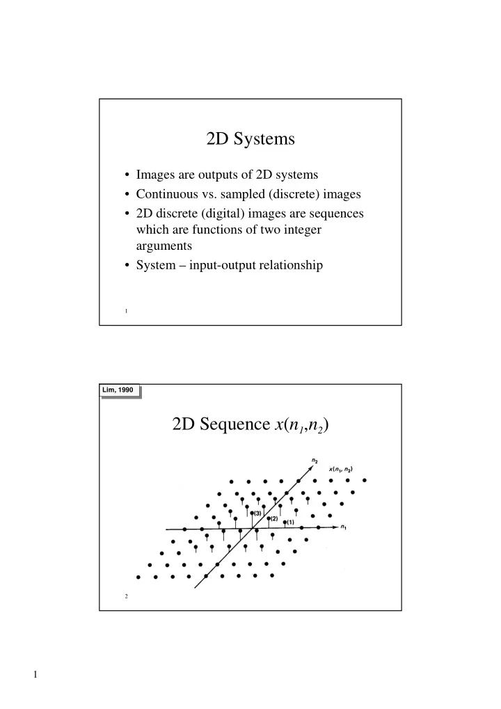
2D Systems • Images are outputs of 2D systems • Continuous vs. sampled (discrete) images • 2D discrete (digital) images are sequences which are functions of two integer arguments • System – input-output relationship 1 Lim, 1990 2D Sequence x ( n 1 , n 2 ) 2 1

Lim, 1990 2D Sequence x ( n 1 , n 2 ) (cont’) 3 Lim, 1990 2D Sequence x ( n 1 , n 2 ) (cont’) 4 2

2D Sequences (cont’) • Impulses = =  1 n n 0 δ = 1 2  ( n , n ) impulse (unit sample sequence) 1 2  0 otherwise =  1 n 0 δ = 1  ( n ) line impulse (T indicates 2D sequence of one variable) T 1  0 otherwise ≥  1 n , n 0 = 1 2  u ( n , n ) unit step sequence 1 2  0 otherwise = x ( n , n ) f ( n ) g ( n ) separable sequence 1 2 1 2 5 Lim, 1990 Impulse δ ( n 1 , n 2 ) 6 3

Sequence Representation as Linear Combination of Shifted Impulses sequence value 7 Lim, 1990 Line Impulse δ T ( n 1 ) 8 4

Lim, 1990 Unit Step Sequence u ( n 1 , n 2 ) 9 Step Sequence u T ( n 1 ) 10 5

Jain, 1989 2D Separable Functions f ( x 1 , x 2 )= f 1 ( x 1 ) f 2 ( x 2 ) 11 Periodic Sequence 12 6

Linear Systems • Input-output relationship is called a system if there is a unique output for any given input [ ] . = y ( n , n ) T x ( n , n ) 1 2 1 2 [ ] ⇔ + = Linearity T ax ( n , n ) bx ( n , n ) • 1 1 2 2 1 2 + ay ( n , n ) by ( n , n ) 1 1 2 2 1 2 which is the principle of superposition . 13 Linear vs. Nonlinear System 14 7

2D Convolution (cont’) = ∗ ≡ y ( n , n ) x ( n , n ) h ( n , n ) 1 2 1 2 1 2 ∞ ∞ ∑ ∑ − − x ( k , k ) h ( n k , n k ) 1 2 1 1 2 2 = −∞ = −∞ ' ' k k 1 2 where ( , ) is the input and x n n 1 2 − − h ( n k , n k ) the impulse response 1 1 2 2 15 Castleman, 1996 1D Convolution by Castleman 16 8

Jain, 1989 2D Convolution by Jain (1) 17 Jain, 1989 2D Convolution by Jain (2) 18 9

Lim, 1990 …and 2D convolution by Lim 19 2D Convolution • Applications � Deconvolution (deblurring due to deformation, motion, atmosphere) � Noise removal � Estimating original signal � Detecting known feature embedded in a noisy background � Feature enhancement (edges, spots) 20 10

Castleman, 1996 Applications 1: Deconvolution 21 Castleman, 1996 Applications 2: Smoothing 22 11

Castleman, 1996 Applications 3: Edge Enhancement 23 Lim, 1990 Region of Convolution 24 12

Lim, 1990 Convolution with a Separable Sequence 25 The Fourier Transform of a 2D Sequence x ( m , n ) • The Fourier Transform Pair ∞ ∞ ∑ ∑ ω ω ≡ − ω + ω π ≤ ω ω < π X ( , ) x ( m , n ) exp{ j ( m n )}, - , 1 2 1 2 1 2 = −∞ = −∞ m n π π 1 ∫ ∫ = ω ω ω + ω ω ω x ( m , n ) X ( , ) exp{ j ( m n )} d d π 1 2 1 2 1 2 2 ( 2 ) ω = − π ω = − π 1 2 26 13

Lim, 1990 Properties of the Fourier Transform by Lim 27 Castleman, 1996 Properties of the Fourier Transform by Castleman 28 14

Properties of the Fourier Transform • The addition theorem (addition in time/spatial domain corresponds to addition in frequency) • The shift theorem (shifting a function causes only to phase shift) • The convolution theorem (convolution is equivalent to multiplication in the other domain) • … 29 Castleman, 1996 The Addition Theorem { } Φ + = f ( t ) g ( t ) ∞ [ ] ∫ + − π 2 j st f ( t ) g ( t ) e dt − ∞ ∞ ∞ ∫ ∫ − π + − π = 2 j st 2 j st f ( t ) e dt g ( t ) e dt − ∞ − ∞ + F ( s ) G ( s ) 30 15

Lim, 1990 The Fourier Transform – Example 1 low-pass � blur 31 Lim, 1990 The Fourier Transform – Example 1 ∞ ∞ ∑ ∑ ω ω = − ω + ω H ( , ) h ( n , n ) exp{ j ( n n )} 1 2 1 2 1 1 2 2 = −∞ = −∞ n n 1 2 1 1 1 1 1 = + − ω + − ω + ω + ω j j j j e e e e 1 2 1 2 3 6 6 6 6 1 1 1 = + ω + ω cos( ) cos( ) 1 2 3 3 3 32 16

Lim, 1990 The Fourier Transform – Example 1 33 Lim, 1990 The Fourier Transform – Example 2 high-pass the sequence is separable ω ω = ω ω H ( , ) H ( ) H ( ) 1 2 1 1 2 2 � = ω ω (3 - 2cos ) (3 - 2cos ) 1 2 34 17

Lim, 1990 The Fourier Transform – Example 2 35 Castleman, 1996 A 2D Fourier Transform 36 18

Lim, 1990 Phase-Only & Magnitude- Only 37 Lim, 1990 Image Synthesis 38 19

Lim, 1990 Iterative Phase-Only 39 The 2D DFT • If g ( i , k ) is an N x N array, then the 2D discrete Fourier transform pair is given by − − i k N 1 N 1 − π + 1 ∑∑ j 2 ( m n ) = G ( m , n ) g ( i , k ) e N N N = = i 0 k 0 − − m n N 1 N 1 π + 1 ∑∑ j 2 ( i k ) = g ( i , k ) G ( m , n ) e N N N = = m 0 n 0 40 20