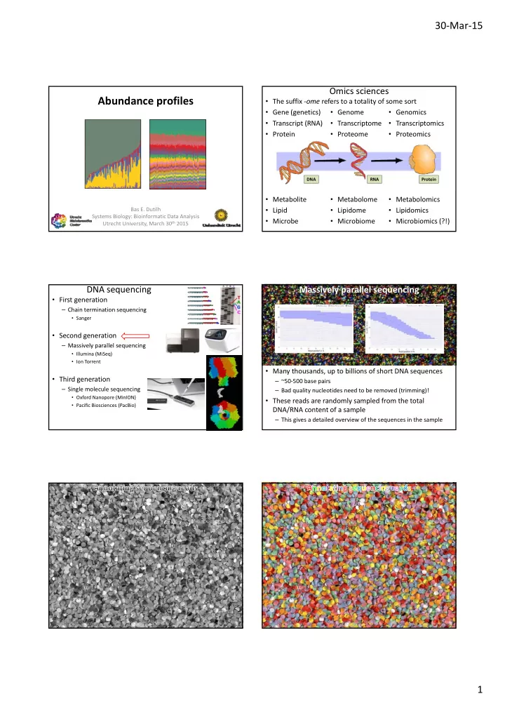
Abundance profiles The suffix ome refers to a totality of some sort - - PDF document

SLIDE 1

30‐Mar‐15 1

Abundance profiles

Bas E. Dutilh Systems Biology: Bioinformatic Data Analysis Utrecht University, March 30th 2015

Omics sciences

• The suffix ‐ome refers to a totality of some sort
• Gene (genetics)
• Transcript (RNA)
• Protein
• Genome
• Transcriptome
• Proteome
• Genomics
• Transcriptomics
• Proteomics

RNA Protein

• Metabolite
• Lipid
• Microbe
• Metabolome
• Lipidome
• Microbiome
• Metabolomics
• Lipidomics
• Microbiomics (?!)

DNA

DNA sequencing

• First generation

– Chain termination sequencing

• Sanger
• Second generation

– Massively parallel sequencing

• Illumina (MiSeq)
• Ion Torrent
• Third generation

– Single molecule sequencing

• Oxford Nanopore (MinION)
• Pacific Biosciences (PacBio)

Massively parallel sequencing

• Many thousands, up to billions of short DNA sequences

– ~50‐500 base pairs – Bad quality nucleotides need to be removed (trimming)!

• These reads are randomly sampled from the total

DNA/RNA content of a sample

– This gives a detailed overview of the sequences in the sample

SLIDE 2

30‐Mar‐15 2

Who/what is present in the sample?

• Last week we discussed how to annotate these

sequencing reads by aligning to a reference database

– Fast, heuristic similarity search programs are used for this

• The result is an overview of the genes/functions/microbes

and their relative abundances in the sequencing reads

High Many reads g Low Many reads Few reads

Functions Species

• r taxa

Micro‐arrays

• Micro‐arrays are another way of identifying sequences in a

sample

– Micro‐arrays can only identify previously known sequences – That is why DNA sequencing is now the standard

A micro‐array is a glass slide that contains pieces of DNA with a known sequence q Green/red labeled sample sequences hydridize to the sequences on the micro‐array

These results are just lists of numbers

• DNA: metagenome: list of all microbial

genes and organisms and relative abundances in an environment

– Micro‐organisms play important roles in ecology and thus in health

• RNA: transcriptome lists all genes and their relative

expression values in a cell/tissue expression values in a cell/tissue

– Gene expression is important for phenotype

• Protein: proteome lists all proteins in a sample and their

relative abundances

– Proteins perform most of the functions in a cell

• A list of numbers is also known as a

multidimensional vector, for example:

ax ay az

DNA: human microbiome

• Which bacterial phyla are present in different

human body sites?

• Which metabolic functions do they encode?
• Can we use this to understand the differences

between people?

Different healthy people

DNA: microbiome studies

Jack Gilbert

Argonne National Lab

Jack Gilbert

Argonne National Lab

RNA: discover cancer biomarker genes

• Can we improve the prognosis for cancer patients by

analyzing their gene expression profile?

Up‐regulated genes Down‐regulated genes

ts

Genes

Patient

SLIDE 3

30‐Mar‐15 3

RNA: heat shock response

• How do Saccharomyces cerevisiae (yeast) genes respond

to increased growth temperature?

Up‐regulated genes Down‐regulated genes

s

5 15 30 60

Time (minutes)

Gene

High‐throughput sequencing

• Same organism, different tissues or body sites

– For example: brain versus liver, mouth versus gut

• Same tissue, same organism

– For example: treatment versus control, tumor versus healthy

• Same tissue, different organisms

– For example: wildtype versus knock‐out/transgenic/mutant, comparing monozygotic twin pairs comparing monozygotic twin pairs

• Time course experiments

– For example: effect of a treatment, development of a tissue, response of microbiota to environmental change

Scaling

• When analyzing transcriptome data, we find that the RNA

expression of gene A consists of:

– 4,000 reads in a healthy tissue sample – 10,000 reads in a tumor sample

• Can we conclude that gene A is over‐expressed in cancer?

– The total volume of the transcriptomic datasets are:

• 80 000 sequencing reads from the healthy tissue

80,000 sequencing reads from the healthy tissue

• 500,000 sequencing reads from the tumor

– No, the gene is actually expressed much lower in the tumor

4,000 80,000 10,000 500,000 = 0.05 = 0.02 Tumor: Healthy:

Comparing read counts

• To compare samples, we need to:

– Scale the numbers so that they add up to 1

• This accounts for differences in the sample size (total number of reads)
• Divide each number by the total number of reads

– Normalize numbers so that they are (close to) normally distributed

• This is important in many statistical tests

Bi l i l d t ft l ith i ll di t ib t d if ld t k

• Biological data are often logarithmically distributed – if so, you could take

the logarithm of the number of reads to normalize Value Log (value)

Gene expression in time

• Normalized and scaled gene expression values

– For example, expression of genes in aging Arabidopsis leaves G 2 Gene 1

15 20 25

pression

0. 0.

Gene 3 Gene 2

5 10 15 1 2 3 4 5 6 7 8 9 10

Abundance/Exp …or leaves… Time/environments/samples…

0. 0. 0.0

SLIDE 4

30‐Mar‐15 4

Microbial abundance in time

• Normalized and scaled microbial abundance values

– For example, presence of pathogens on rotting Arabidopsis leaves Mi b 2 Microbe 1

15 20 25

pression

0. 0.

Microbe 3 Microbe 2

5 10 15 1 2 3 4 5 6 7 8 9 10

Abundance/Exp Time/environments/samples… …or leaves…

0. 0. 0.0

Research setup

• 1. Design experimental conditions and sampling strategy
• 2. Extract DNA/RNA/protein
• 3. Sequence nucleotides or proteins
• 4. Quality control of sequencing reads or peptides
• 5. Annotate (e.g. align reads to database) and count
• 6. Normalize and scale the counts
• 7. Compare samples, clustering (next lecture)
• 8. Interpret results and perform verification experiments

Quantifying similarity between vectors

• Based on these measurements, which genes/microbes/etc are more

similar to each other?

15 20 25

pression

• Abundance/expression levels

are most similar between and

• Abundance/expression patterns

are most similar between and W di t

0. 0. 5 10 15 1 2 3 4 5 6 7 8 9 10

Abundance/Exp Time/Environments/Samples

• We can use a distance measure

to quantify the (dis‐)similarity between the lists – Many different distance measures exist

0. 0. 0.0

Distance matrices

• Distance matrix

x y x z y z

• Similarity matrix

1 1 ‐ x 1 ‐ y 1 ‐ x 1 1 ‐ z 1 ‐ y 1 ‐ z 1

inverse inverse

distance = 1 ‐ similarity

Manhattan distance (levels)

0.265 0.265 0.799 0.799 0.534 0.534

• Example:

d = |0.20 – 0.15| + dAB = |XA – XB| + |YA – YB|

1 0.20 0.15 0.12 2 0.17 0.15 0.09 3 0.16 0.16 0.08 4 0.20 0.15 0.11 5 0.20 0.16 0.12 6 0.17 0.16 0.10 7 0.16 0.15 0.08 8 0.20 0.15 0.12 9 0.18 0.16 0.11 10 0.16 0.15 0.08

|0.17 – 0.15| + |0.16 – 0.16| + |0.20 – 0.15| + |0.20 – 0.16| + |0.17 – 0.16| + |0.16 – 0.15| + |0.20 – 0.15| + |0.18 – 0.16| + |0.16 – 0.15| = 0.265 d = 0.799 d = 0.534

(YA – YB)2 dAB

2

= +

Euclidean distance (levels)

0.103 0.103 0.253 0.253 0.178 0.178

• Example:

d 2 = (0.20 – 0.15)2 +

(YA – YB)2 dAB

2

dAB = (XA – XB)2 + (YA – YB)2

( A

B)

(XA – XB)2

(0.17 – 0.15)2 + (0.16 – 0.16)2 + (0.20 – 0.15)2 + (0.20 – 0.16)2 + (0.17 – 0.16)2 + (0.16 – 0.15)2 + (0.20 – 0.15)2 + (0.18 – 0.16)2 + (0.16 – 0.15)2 = 0.0105  d = 0.103 d = 0.253 d = 0.178

( A

B)

(XA – XB)2 1 0.20 0.15 0.12 2 0.17 0.15 0.09 3 0.16 0.16 0.08 4 0.20 0.15 0.11 5 0.20 0.16 0.12 6 0.17 0.16 0.10 7 0.16 0.15 0.08 8 0.20 0.15 0.12 9 0.18 0.16 0.11 10 0.16 0.15 0.08

SLIDE 5

30‐Mar‐15 5

0.15 0.2 0.25

ression

Comparing patterns instead of distances

• Correlation can be used to quantify the similarity between

patterns

r = ‐0.35 Low correlation 1 0.20 0.15 0.12 2 0.17 0.15 0.09 3 0.16 0.16 0.08 4 0.20 0.15 0.11 5 0.20 0.16 0.12 6 0.17 0.16 0.10 0.05 0.1 0.05 0.1 0.15 0.2 0.25

Abundance/Exp Abundance/Expression of 1 1 1

0.97 0.97 ‐0.35 ‐0.35 ‐0.16 ‐0.16 1.35 1.35 1.16 1.16 0.03 0.03

r = 0.97 High correlation 7 0.16 0.15 0.08 8 0.20 0.15 0.12 9 0.18 0.16 0.11 10 0.16 0.15 0.08 0 15 0.2 0.25

ession 1 1 1

0.97 0.97 ‐0.35 ‐0.35 ‐0.16 ‐0.16 1.35 1.35 1.16 1.16 0.03 0.03

Compare patterns instead of distances

• Correlation can be used to quantify

the similarity between patterns

15 20 25

pression

0. 0. r = ‐0.35 Little correlation 0.05 0.1 0.15 0.05 0.1 0.15 0.2 0.25

Abundance/Expr Abundance/Expression of

5 10 15 1 2 3 4 5 6 7 8 9 10

Abundance/Exp Time/Environments/Samples

0. 0. 0.0 r = 0.97 Positive correlation