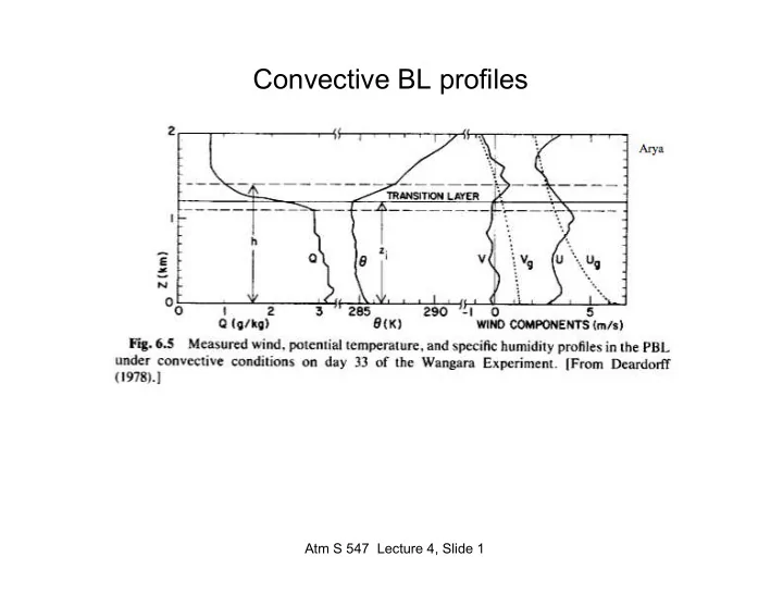
Convective BL profiles Atm S 547 Lecture 4, Slide 1 Moderately - - PowerPoint PPT Presentation

Atm S 547 Lecture 4, Slide 1

Convective BL profiles

Atm S 547 Lecture 4, Slide 2

Moderately stable BL profiles

Atm S 547 Lecture 4, Slide 3

Highly stable BL profiles

Wind hodograph at South Pole Station Categories 1-8 correspond to increasingly stable BLs; dots are composites of measurements at 0.5, 1, 2, 4, 8, 12, 16, 20, 24, 32 m; y-axis is in the surface wind direction. Note large turning of the wind with height in stable BLs.

ABL observing technologies - Surface measurements

Surface measurements

• Sonic anemometers (fast-response air velocity), ocean buoys
• Fast-response temperature, humidity, gas sensors
• Surface meteorology, chemistry, aerosols
• Downward radiation

Atm S 547 Lecture 4, Slide 4

Sonic + gas analyzer for eddy-correlation CO2 flux Sonic anemometer Pyranometer

ABL obs - Remote sensing

• Doppler lidar (aerosol scattering), ceilometers, nephelometers
• mm-wavelength radar (cloud scattering)
• Sodar and 915 MHz wind profilers
• RASS (virtual temperature profiling via Bragg scattering of radar waves

from sound-induced density anomalies moving away at sound speed)

Atm S 547 Lecture 4, Slide 5

Phased-array Doppler sodar (ABL wind profiling) RASS + wind profiler Doppler lidar

ABL obs - Specialized platforms

• Flux towers for measurements at multiple heights
• Tethered balloons
• Aircraft/helicopter

Atm S 547 Lecture 4, Slide 6

Cabauw 220 m flux tower, NL Robotic helicopter with gas-sensing instrumentation

Large eddy simulation (e. g. SAM or WRF)

• Discretize and solve 3D compressible or Boussinesq fluid

equations on a grid.

• Grid spacing << size of most energetic eddies

(typically 5 -50 m in vertical, 1-5x larger in horizontal)

• Horizontal domain size > size of most energetic eddies

(typically 2 km (stable BL) – 20 km (convective BLs w

• Typically use horizontally periodic boundary conditions
• Advect potl. temp, other quantities of interest, (moisture,

chemical constituents) using sophisticated schemes that minimize spurious oscillations, maintain accuracy

• Subgrid turbulence scheme (‘Smagorinsky’ eddy diffusion)
• Other relevant physics (surface fluxes, radiation, clouds)
• Effects of large-scale advection added if periodic BCs used

Atm S 547 Lecture 4, Slide 7

Atm S 547 Lecture 4, Slide 8

LES of atmospheric boundary layer

Application I: Visualization See class web-page links to animations of LES-simulated: Sc-capped BL (4x4 km, courtesy B. Stevens, UCLA):

• Vertical cross-section of w
• horizontal view of cloud albedo

Cu rising into Sc (6x6 km, courtesy I. Sandu, ECMWF) (white is cloud; grey blobs are rain)

Atm S 547 Lecture 4, Slide 9

Application II: Turbulence fluxes and statistics

Stevens et al. 2005

Atm S 547 Lecture 4, Slide 10

Application III: Parameterization development/testing

GABLS-1 idealized stable boundary layer (Beare et al. 2006)

• Stable stratification,

Vg = 10 m s-1

• Surface cooled at 0.25

K hr-1 for 9 hrs.

• Several LESs run with

3 m resolution.

• Compared with new

(UW) and existing PBL parameterizations in NCAR’s CAM3 climate model.

• New and modified

schemes clearly

• utperform current

approach compared to LES for this case.

Bretherton and Park (2009 J.Clim)