A Unified Bias-Variance Decomposition and its Applications Pedro - PDF document

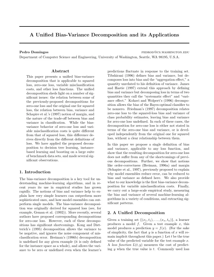
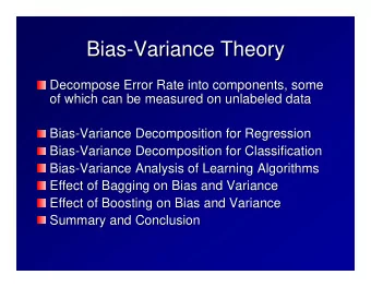
A Unified Bias-Variance Decomposition and its Applications Pedro Domingos pedrod@cs.washington.edu Department of Computer Science and Engineering, University of Washington, Seattle, WA 98195, U.S.A. Abstract predictions fluctuate in response to the training set. Tibshirani (1996) defines bias and variance, but de- This paper presents a unified bias-variance composes loss into bias and the “aggregation effect,” a decomposition that is applicable to squared quantity unrelated to his definition of variance. James loss, zero-one loss, variable misclassification and Hastie (1997) extend this approach by defining costs, and other loss functions. The unified bias and variance but decomposing loss in terms of two decomposition sheds light on a number of sig- quantities they call the “systematic effect” and “vari- nificant issues: the relation between some of ance effect.” Kohavi and Wolpert’s (1996) decompo- the previously-proposed decompositions for sition allows the bias of the Bayes-optimal classifier to zero-one loss and the original one for squared be nonzero. Friedman’s (1997) decomposition relates loss, the relation between bias, variance and zero-one loss to the squared-loss bias and variance of Schapire et al.’s (1997) notion of margin, and class probability estimates, leaving bias and variance the nature of the trade-off between bias and for zero-one loss undefined. In each of these cases, the variance in classification. While the bias- decomposition for zero-one loss is either not stated in variance behavior of zero-one loss and vari- terms of the zero-one bias and variance, or is devel- able misclassification costs is quite different oped independently from the original one for squared from that of squared loss, this difference de- loss, without a clear relationship between them. rives directly from the different definitions of loss. We have applied the proposed decom- In this paper we propose a single definition of bias position to decision tree learning, instance- and variance, applicable to any loss function, and based learning and boosting on a large suite show that the resulting decomposition for zero-one loss of benchmark data sets, and made several sig- does not suffer from any of the shortcomings of previ- nificant observations. ous decompositions. Further, we show that notions like order-correctness (Breiman, 1996a) and margin (Schapire et al., 1997), previously proposed to explain 1. Introduction why model ensembles reduce error, can be reduced to bias and variance as defined here. We also provide The bias-variance decomposition is a key tool for un- what to our knowledge is the first bias-variance decom- derstanding machine-learning algorithms, and in re- position for variable misclassification costs. Finally, cent years its use in empirical studies has grown we carry out a large-scale empirical study, measuring rapidly. The notions of bias and variance help to ex- the bias and variance of several machine-learning al- plain how very simple learners can outperform more gorithms in a variety of conditions, and extracting sig- sophisticated ones, and how model ensembles can out- nificant patterns. perform single models. The bias-variance decomposi- tion was originally derived for squared loss (see, for example, Geman et al. (1992)). More recently, several 2. A Unified Decomposition authors have proposed corresponding decompositions Given a training set { ( x 1 , t 1 ) , . . . , ( x n , t n ) } , a learner for zero-one loss. However, each of these decompo- produces a model f . Given a test example x , this sitions has significant shortcomings. Kong and Diet- model produces a prediction y = f ( x ). (For the sake terich’s (1995) decomposition allows the variance to of simplicity, the fact that y is a function of x will re- be negative, and ignores the noise component of mis- main implicit throughout this paper.) Let t be the true classification error. Breiman’s (1996b) decomposition value of the predicted variable for the test example x . is undefined for any given example (it is only defined A loss function L ( t, y ) measures the cost of predict- for the instance space as a whole), and allows the vari- ing y when the true value is t . Commonly used loss ance to be zero or undefined even when the learner’s

functions are squared loss ( L ( t, y ) = ( t − y ) 2 ), absolute under squared loss is the mean of the predictions; un- loss ( L ( t, y ) = | t − y | ), and zero-one loss ( L ( t, y ) = 0 der absolute loss it is the median; and under zero-one if y = t , L ( t, y ) = 1 otherwise). The goal of learning loss it is the mode (i.e., the most frequent prediction). can be stated as producing a model with the smallest For example, if there are k training sets in D , we learn possible loss; i.e., a model that minimizes the average a classifier on each, 0 . 6 k of these classifiers predict class L ( t, y ) over all examples, with each example weighted 1, and 0 . 4 k predict 0, then the main prediction under by its probability. In general, t will be a nondetermin- zero-one loss is class 1. The main prediction is not nec- istic function of x (i.e., if x is sampled repeatedly, dif- essarily a member of Y ; for example, if Y = { 1 , 1 , 2 , 2 } ferent values of t will be seen). The optimal prediction the main prediction under squared loss is 1.5. y ∗ for an example x is the prediction that minimizes We can now define bias and variance as follows. E t [ L ( t, y ∗ )], where the subscript t denotes that the ex- pectation is taken with respect to all possible values of Definition 2 The bias of a learner on an example x t , weighted by their probabilities given x . The optimal is B ( x ) = L ( y ∗ , y m ) . model is the model for which f ( x ) = y ∗ for every x . In general, this model will have non-zero loss. In the In words, the bias is the loss incurred by the main case of zero-one loss, the optimal model is called the prediction relative to the optimal prediction. Bayes classifier , and its loss is called the Bayes rate . Definition 3 The variance of a learner on an exam- Since the same learner will in general produce differ- ple x is V ( x ) = E D [ L ( y m , y )] . ent models for different training sets, L ( t, y ) will be a function of the training set. This dependency can be In words, the variance is the average loss incurred by removed by averaging over training sets. In particular, predictions relative to the main prediction. Bias and since the training set size is an important parameter variance may be averaged over all examples, in which of a learning problem, we will often want to average case we will refer to them as average bias E x [ B ( x )] and over all training sets of a given size. Let D be a set average variance E x [ V ( x )]. of training sets. Then the quantity of interest is the It is also convenient to define noise as follows. expected loss E D,t [ L ( t, y )], where the expectation is taken with respect to t and the training sets in D (i.e., Definition 4 The noise of an example x is N ( x ) = with respect to t and the predictions y = f ( x ) pro- E t [ L ( t, y ∗ )] . duced for example x by applying the learner to each training set in D ). Bias-variance decompositions de- In other words, noise is the unavoidable component of compose the expected loss into three terms: bias, vari- the loss, incurred independently of the learning algo- ance and noise. A standard such decomposition exists rithm. for squared loss, and a number of different ones have Definitions 2 and 3 have the intuitive properties associ- been proposed for zero-one loss. ated with bias and variance measures. y m is a measure In order to define bias and variance for an arbitrary of the “central tendency” of a learner. (What “central” loss function we first need to define the notion of main means depends on the loss function.) Thus B ( x ) mea- prediction. sures the systematic loss incurred by a learner, and V ( x ) measures the loss incurred by its fluctuations Definition 1 The main prediction for a loss func- around the central tendency in response to different is y L,D tion L and set of training sets D = training sets. If the loss function is nonnegative then m argmin y ′ E D [ L ( y, y ′ )] . bias and variance are also nonnegative. The bias is in- dependent of the training set, and is zero for a learner When there is no danger of ambiguity, we will repre- that always makes the optimal prediction. The vari- sent y L,D simply as y m . The expectation is taken with ance is independent of the true value of the predicted m respect to the training sets in D , i.e., with respect to variable, and is zero for a learner that always makes the predictions y produced by learning on the training the same prediction regardless of the training set. The sets in D . Let Y be the multiset of these predictions. only property that the definitions above require of the (A specific prediction y will appear more than once in loss function is that its expected value be computable. Y if it is produced by more than one training set.) In However, it is not necessarily the case that the ex- words, the main prediction is the value y ′ whose aver- pected loss E D,t [ L ( t, y )] for a given loss function L age loss relative to all the predictions in Y is minimum can be decomposed into bias and variance as defined (i.e., it is the prediction that “differs least” from all the above. Our approach will be to propose a decomposi- predictions in Y according to L ). The main prediction tion and then show that it applies to each of several