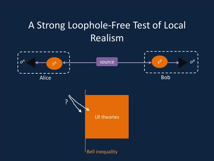
A Strong Loophole-Free Test of Local Realism o A o B s B source s A - - PowerPoint PPT Presentation

A Strong Loophole-Free Test of Local Realism

source sA sB

Alice Bob

• A
• B

LR theories

?

Bell inequality

arXiv:1511.03189 [quant-ph] Lynden K. Shalm, Evan Meyer-Scott, Bradley G. Christensen, Peter Bierhorst, Michael A. Wayne, Martin J. Stevens, Thomas Gerrits, Scott Glancy, Deny R. Hamel, Michael S. Allman, Kevin J. Coakley, Shellee D. Dyer, Carson Hodge, Adriana E. Lita, Varun B. Verma, Camilla Lambrocco, Edward Tortorici, Alan L. Migdall, Yanbao Zhang, Daniel R. Kumor, William H. Farr, Francesco Marsili, Matthew D. Shaw, Jeffrey A. Stern, Carlos Abellán, Waldimar Amaya, Valerio Pruneri, Thomas Jennewein, Morgan W. Mitchell, Paul G. Kwiat, Joshua C. Bienfang, Richard P. Mirin, Emanuel Knill, and Sae Woo Nam

Outline

• Introduction to tests of LR

– History lesson: hidden variables and LR – Bell inequalities

• Hypothesis test of LR

– P-values for LR

• Experiments

– Requirements and loopholes – Past experiments – Our experiment

• Computing our p-values
• Randomness expansion

History Lesson

• In 1920’s some physicists thought that quantum theory was

very strange. – Superposition! – Entanglement! – “Spooky actions!” – Randomness! (not even respectable randomness like in statistical mechanics)

Hidden Variables

• Maybe all of this strangeness could be fixed with “hidden

variables”.

• If we knew the hidden variables, we would be able to predict

the outcomes of all measurements with certainty.

• The quantum randomness would be respectable.
• In 1927 de Broglie invented the pilot wave theory [J. Phys.

Radium].

[images from Bush, Ann. Rev. Fluid Mech., 2015]

Hidden Variables

• Maybe all of this strangeness could be fixed with “hidden

variables”.

• If we knew the hidden variables, we would be able to predict

the outcomes of all measurements with certainty.

• The quantum randomness would be respectable.
• In 1927 de Broglie invented the pilot wave theory [J. Phys.

Radium].

• In 1952 David Bohm completed the pilot wave theory [Phys.

Rev.].

• Bohm’s theory gives exactly the same measurable predictions

as standard non-relativistic quantum theory.

Hidden Variables

• Maybe all of this strangeness could be fixed with “hidden

variables”.

• If we knew the hidden variables, we would be able to predict

the outcomes of all measurements with certainty.

• The quantum randomness would be respectable.
• In 1927 de Broglie invented the pilot wave theory [J. Phys.

Radium].

• In 1952 David Bohm completed the pilot wave theory [Phys.

Rev.].

• Bohm’s theory gives EXACTLY THE SAME MEASURABLE

PREDICTIONS as standard non-relativistic quantum theory.

Hidden Variables

• de Broglie’s and Bohm’s hidden variables are non-local.

– Hidden location of particle can change instantly because of distant events. – Hidden particle can travel faster than light.

Hidden Variables

• Bell wrote:

– Bohm of course was well aware of these features of his scheme, and has given them much attention. However, it must be stressed that, to the present writer's knowledge, there is no proof that any hidden variable account of quantum mechanics must have this extraordinary

• character. It would therefore be interesting, perhaps, to

pursue some further "impossibility proofs". [Rev. Mod. Phys., 1966]

• Need a mathematical formulation.

Local Realism

• Realism: all systems have pre-existing values for all possible

measurements. – even incompatible measurements.

• Local realism: pre-existing values depend only on events in

the past lightcone of the system.

• Classical physics obeys LR.
• Does quantum physic obey LR?

[Image source: K. Aainsqatsi at Wikipedia]

Bell’s Inequalities

• Bell’s thought experiment:
• Alice and Bob randomly choose measurements sA{a, a’} and

sB{b, b’}.

• They get outcomes oA, oB{0,+}.
• LR constrains P(oA, oB | sA, sB).
• Bell found an inequality that is obeyed by all LR P(oA, oB | sA,

sB), but is violated by some entangled quantum systems [Physics, 1964].

source sA sB

Alice Bob

• A
• B

Bell’s Inequalities

• A marginal problem:

– LR outcome random variables dA

a, dA a’, dB b, dB b’.

– Physicists measure marginals

• P(dA

a, dB b | a, b)

• P(dA

a, dB b’| a, b’)

• P(dA

a’, dB b| a’, b)

• P(dA

a’, dB b’ | a’, b’)

– Are these compatible with P(dA

a, dB b, dA a’, dB b’, sA, sB)?

– If “no”, LR is false.

source sA sB

Alice Bob

• A
• B

Distance-Based Bell Inequalities

• Use triangle inequality to construct Bell inequalities:

[Shumacher, PRA, 1991]

• Deterministic LR model gives outcomes for all settings

– dLR=(dA

a, dA a’, dB b, dB b’)

LR outcome space dA

a

dB

b’

dB

b

dA

a’

Distance-Based Bell Inequalities

• Use triangle inequality to construct Bell inequalities:

[Shumacher, PRA, 1991]

• Deterministic LR model gives outcomes for all settings

– dLR=(dA

a, dA a’, dB b, dB b’)

• Pseudo-distance: l(x,y) obeys triangle inequality

l(dA

a’ ,dB b) + l(dB b ,dA a) + l(dA a ,dB b’) - l(dA a’ ,dB b’) ≥ 0

LR outcome space dB

b’

dB

b

dA

a’

dA

a

Distance-Based Bell Inequalities

• l(dA

a’ ,dB b) + l(dB b ,dA a) + l(dA a ,dB b’) - l(dA a’ ,dB b’) ≥ 0

• dLR=(dA

a, dA a’, dB b, dB b’) is hidden, but for any P(dLR)

E[l(dA

a’ ,dB b)] + E[l(dB b ,dA a)] + E[l(dA a,dB b’)] – E[l(dA a’ ,dB b’)] ≥ 0

– A constraint that the global distribution places on the marginals.

Bell Inequality

Distance-Based Bell Inequalities

• E[l(dA

a’ ,dB b)] + E[l(dB b ,dA a)] + E[l(dA a,dB b’)] – E[l(dA a’ ,dB b’)] ≥ 0

• Example: outcomes dX

c{-1,1}

– l(x,y) = ½|yx|  CHSH Inequality [Clauser et al., PRL, 1969] E[oAoB|a,b]+E[oAoB|a,b’]+E[oAoB|a’,b] - E[oAoB|a’,b’] ≤ 2

• Many other possibilities:

– Other pseudo-distance functions l(x,y) – Only constraint: l(x,y) obeys triangle inequality

LR Polytope

• All the Bell inequalities make a polytope

LR theories

Bell inequality

LR Polytope

• All the Bell inequalities make a polytope.
• Quantum theories allow stronger correlations.

LR theories

Bell inequality

Quantum theories

Outline

• Introduction to tests of LR

– History lesson: hidden variables and LR – Bell inequalities

• Hypothesis test of LR

– P-values for LR

• Experiments

– Requirements and loopholes – Past experiments – Our experiment

• Computing our p-values
• Randomness expansion

Hypothesis Test of Local Realism

• Does quantum theory obey LR?
• Does reality obey LR?
• Do experiment.
• Get counts N(oA, oB | sA, sB)  oA, oB , sA, sB.
• How certain are we that our counts were not caused by an LR

system? LR theories ?

Bell inequality

NO Use statistics!

Hypothesis Test of Local Realism

• Test of LR as a Hypothesis Test:

– Null Hypothesis H0: “Experiment obeys LR & X & Y…” – Do n trials; get results (o1,o2,…,on) – Compute test statistic: Tobs(o1,o2,…,on) – P-value = supLR[PLR (T Tobs)] – Smaller p-value is stronger evidence against H0.

• How to compute p-values for LR tests?

– Gill [quant-ph/0301059]; Zhang, Glancy, and Knill’s PBR [arXiv:1108.2468, 1303.7464]; Bierhorst [1311.3605, 1311.3605]; Kofler et al. [1411.4787]; Elkouss and Wehner [1510.07233].

P-value Cartoon T maxTLR TQM

P-value Cartoon T maxTLR TQM P(T)QM P(T)LR

P-value Cartoon T maxTLR TQM P(T)QM P(T)LR Tobs

P-value Cartoon T maxTLR TQM P(T)QM P(T)LR Tobs

p-value

Outline

• Introduction to tests of LR

– History lesson: hidden variables and LR – Bell inequalities

• Hypothesis test of LR

– P-values for LR

• Experiments

– Requirements and loopholes – Past experiments – Our experiment

• Computing our p-values
• Randomness expansion

Experiments and Loopholes

• Experiments need:

– Well defined trials

• Choose random setting, get outcomes

– Independence of choices – Isolation of measurement stations

• Spacelike separation of choices from remote

measurement. – High efficiency transmission and measurements

•  > 2/3

– High fidelity entangled particles – Rigorous analysis

• without assuming i.i.d. and normal distribution

Experiments and Loopholes

• Experiments are not perfect.
• Loophole: way that LR system can violate a Bell inequality in

an experiment. – Experiment does not meet requirements. – Assumptions that can’t be verified

• About device
• During analysis

Past Experiments

• Many past experiments – all had loopholes.
• Loopholes have closed as technology improved:
• S. J. Freedman and J. F. Clauser, Phys. Rev.
• Lett. 28, 938 (1972).
• A. Aspect, P. Grangier, and G. Roger, Phys.
• Rev. Lett. 47, 460 (1981).
• A. Aspect, P. Grangier, and G. Roger, Phys.
• Rev. Lett. 49, 91 (1982).
• A. Aspect, J. Dalibard, and G. Roger, Phys.
• Rev. Lett. 49, 1804 (1982).
• G. Weihs, T. Jennewein, C. Simon, H.

Weinfurter, and A. Zeilinger, Phys. Rev. Lett. 81, 5039 (1998).

• M. A. Rowe, D. Kielpinski, V. Meyer, C. A.

Sackett, W. M. Itano, C. Monroe, and D. J. Wineland, Nature 409, 791 (2001).

• T. Scheidl, R. Ursin, J. Kofler, S. Ramelow, X.-
• S. Ma,T. Herbst, L. Ratschbacher, A. Fedrizzi,
• N. K. Langford, T. Jennewein, and A. Zeilinger,
• Proc. Nat. Acad. Sci. USA 107, 19708 (2010).
• M. Giustina, A. Mech, S. Ramelow, B.

Wittmann, J. Kofler, J. Beyer, A. Lita, B. Calkins, T. Gerrits, S. W. Nam, R. Ursin, and A. Zeilinger, Nature 497, 227 (2013)

• B. G. Christensen, K. T. McCusker, J. B.

Altepeter, B. Calkins, T. Gerrits, A. E. Lita, A. Miller, L. K. Shalm, Y . Zhang, S. W. Nam, N. Brunner, C. C. W. Lim, N. Gisin, and P. G. Kwiat, Phys. Rev. Lett. 111, 130406 (2013).

3 New Experiments

• In 2015, 3 “loophole free” experiments were performed
• B. Hensen, and others, “Loophole-free Bell inequality violation

using electron spins separated by 1.3 kilometres” Nature. At TU Delft. – P-value = 0.039.

3 New Experiments

• In 2015, 3 “loophole free” experiments were performed
• B. Hensen, and others, “Loophole-free Bell inequality violation

using electron spins separated by 1.3 kilometres” Nature. At TU Delft. – P-value = 0.039.

3 New Experiments

• In 2015, 3 “loophole free” experiments were performed
• B. Hensen, and others, “Loophole-free Bell inequality violation

using electron spins separated by 1.3 kilometres” Nature. At TU Delft. – P-value = 0.039.

• M. Giustina and others, “Significant-Loophole-Free Test of

Bell’s Theorem with Entangled Photons” Phys. Rev. Lett. At University of Vienna. – P-value = 3.74×10-31.

3 New Experiments

• In 2015, 3 “loophole free” experiments were performed
• B. Hensen, and others, “Loophole-free Bell inequality violation

using electron spins separated by 1.3 kilometres” Nature. At TU Delft. – P-value = 0.039.

• M. Giustina and others, “Significant-Loophole-Free Test of

Bell’s Theorem with Entangled Photons” Phys. Rev. Lett. At University of Vienna. – P-value = 3.74×10-31.

• K. Shalm and others, “Strong Loophole-Free Test of Local

Realism” Phys. Rev. Lett. At NIST-Boulder. – P-value = 2.3×10-7.

Our Experiment

Source makes entangled state: 0.995|HH+0.276ei|VV by SPDC into fibers.

Superconducting Nanowire Single Photon Detector

• Detector efficiency  90 %
• Total transmission and detection efficiency  75 %
• Latency  11 ns, Jitter 150 ps. [Marsili and others,

arXiv:1209.5774]

Timing

Timing

Outline

• Introduction to tests of LR

– History lesson: hidden variables and LR – Bell inequalities

• Hypothesis test of LR

– P-values for LR

• Experiments

– Requirements and loopholes – Past experiments – Our experiment

• Computing our p-values
• Randomness expansion

How We Compute P-values

• Define “trial”:

– Fixed time window after synch pulse arrives at Alice and Bob. – When they are ready. – Measurement choices. – Detector click times.

• Convert detection timetags to 0/+ outcomes

– “0” if no photons detected – “+” if any photons detected

Binomial Method

• See Bierhorst [arXiv:1312.2999].
• For the CH inequality:

– P(++|ab)  P(+0|ab’) + P(0+|a’b) + P(++|a’b’) – Does not include 00 terms – less sensitive to failed downconversion.

• Consider subsequence of trials with outcomes C = {++ab,

+0ab’, 0+a’b, ++a’b’}.

• If ++ab  HEADS, otherwise TAILS.
• Under optimal LR model, coin flips have binomial distribution

with P(HEADS) = ½.

• P-value = probability to get at least observed # of HEADS using

a fair coin.

Binomial Method

• For valid p-values, we must choose a stopping criterion in

advance.

• Actual experiment was done for fixed amount of time.
• Warning: # of C={++ab, +0ab’, 0+a’b, ++a’b’} outcomes is

random.

• Use initial data to estimate rate of C outcomes.
• Choose NC to be analyzed from remainder of data.

Waiting for GPS signal. Estimate rate of C’s. Choose Nc Contains NC trials with C

• utcomes

Discard t = 0 t = 30 min

Binomial Method

• For “Classical XOR 3” data set:
• Total trials = 182,137,032
• Nc = 12,127
• # of HEADS = 6,378
• p-value = 5.8510-9

RNG Bias Correction

• What if RNGs have bias: P(a)  P(a’)  ½ or P(b)  P(b’)  ½?
• How should we adjust p-values?
• Define excess predictability bound

–  = 2 max[P(a), P(a’), P(b), P(b’)] – 1

• Under the optimal LR theory,   0 allows

– P(HEADS) 

1 2 + 𝜁 1+𝜁2.

– If ε ≤ 3×10-3, p-value ≤ 2.3×10-7,

P-value: Best Practice

• P-value: Given a test statistic, the p-value is the probability,

according to null hypothesis, of observing a test statistic value as or more extreme than the observed value.

• For probability statement to hold, one must

– Commit to analysis method. – Choose stopping rule. – Take data. – Compute p-value. – Publish p-value (whatever it is).

P-value: What We Did

• Took several data sets.
• Chose good stopping rules in advance.
• Tried different analysis methods.

– PBR [Zhang, Glancy, Knill, arXiv:1108.2468] – Binomial – Adjusted trail duration

• In supplementary material, we gave a big table of p-values.

P-value What We Did

• Took several data sets.
• Chose good stopping rules in advance.
• Tried different analysis methods.

– PBR [Zhang, Glancy, Knill, arXiv:1108.2468] – Binomial – Adjusted trial duration

• In supplementary material, gave a giant table of p-values.

– Informative, but difficult to interpret. – How to combine into a single p-value? ¯\_(ツ)_/¯

• Abstract says “p-values as low as 5.910-9”.

P-value What We Did

• Rigor of p-values is slightly weakened by exploratory analysis.

– Typical of most physics experiments. – # of analysis decisions is not very large. – Most important analysis decisions were made on training data sets.

• Hopefully our p-values are small enough that they still provide

good evidence against LR.

Outline

• Introduction to tests of LR

– History lesson: hidden variables and LR – Bell inequalities

• Hypothesis test of LR

– P-values for LR

• Experiments

– Requirements and loopholes – Past experiments – Our experiment

• Computing our p-values
• Randomness expansion

Randomness Expansion

• Secure randomness generation

– For NIST random beacon – Broadcasts 512 bits every minute for public use.

Randomness Expansion

• Secure randomness generation

– Let’s use a test of local realism as the entropy source! – Why? – An LR system has hidden variables that predict measurement outcomes. – A hacker is like a hidden variable. – If we can reject LR, we reject hackers’ ability to predict.

Randomness Expansion

• Peter Bierhorst, Lynden K. Shalm, Alan Mink, Stephen Jordan,

Yi-Kai Liu, Andrea Rommal, Scott Glancy, Bradley Christensen, Sae Woo Nam, and Emanuel Knill

• Theory project: lower-bound min-entropy as a function of Bell

inequality violation. – Needed protocol robust to noisy experiment that barely violates.

• Software project: extract unbiased bits from Bell test output.

– Trevisan extractor – Fixed and optimized code of Mauerer, Portmann, and Scholz (arXiv:1212:.0520).

Randomness Expansion

• We made 256 random bits, uniform to within 0.001:

1011000000101000101000011010100111001010110000111001 0100111011111001101101100010011110100101010100101001 1001011011100110001010010000100001011000100100101111 1100110010000001111111100011101111000111101101110110 001100100001110101001100100101010000111101010100

FAQ

• No loopholes at all? Really?
• Have you thought of doing a Bayesian analysis?
• So, now we will never have to hear about tests of LR ever

again!

• Didn’t you use random numbers to make random numbers?
• If nature is not local-realistic, what is it?

Bonus Slides

Lynden K. Shalm,1 Evan Meyer-Scott,2 Bradley G. Christensen,3 Peter Bierhorst,1 Michael A. Wayne,3, 4 Martin J. Stevens,1 Thomas Gerrits,1 Scott Glancy,1 Deny R. Hamel,5 Michael S. Allman,1 Kevin J. Coakley,1 Shellee D. Dyer,1 Carson Hodge,1 Adriana E. Lita,1 Varun B. Verma,1 Camilla Lambrocco,1 Edward Tortorici,1 Alan L. Migdall,4, 6 Yanbao Zhang,2 Daniel R. Kumor,3 William H. Farr,7 Francesco Marsili,7 Matthew D. Shaw,7 Jeffrey A. Stern,7 Carlos Abellán,8 Waldimar Amaya,8 Valerio Pruneri,8, 9 Thomas Jennewein,2, 10 Morgan W. Mitchell,8, 9 Paul G. Kwiat,3 Joshua C. Bienfang,4, 6 Richard P. Mirin,1 Emanuel Knill,1 and Sae Woo Nam1

• 1. National Institute of Standards and Technology, 325 Broadway, Boulder, CO 80305, USA
• 2. Institute for Quantum Computing and Department of Physics and Astronomy, University of

Waterloo, 200 University Ave West, Waterloo, Ontario, Canada, N2L 3G1

• 3. Department of Physics, University of Illinois at Urbana-Champaign, Urbana, IL 61801, USA
• 4. National Institute of Standards and Technology, 100 Bureau Drive, Gaithersburg, MD 20899,USA
• 5. Département de Physique et d'Astronomie, Université de Moncton, Moncton, New Brunswick

E1A 3E9, Canada

• 6. Joint Quantum Institute, National Institute of Standards and Technology and University of

Maryland, 100 Bureau Drive, Gaithersburg, Maryland 20899, USA

• 7. Jet Propulsion Laboratory, California Institute of Technology, 4800 Oak Grove Drive, Pasadena,

CA 91109

• 8. ICFO - Institut de Ciencies Fotoniques, The Barcelona Institute of Science and Technology,

08860 Castelldefels (Barcelona), Spain

• 9. ICREA - Institució Catalana de Recerca i Estudis Avancats, 08015 Barcelona, Spain

10.Quantum Information Science Program, Canadian Institute for Advanced Research, Toronto, ON, Canada

P-value Cartoon T maxTLR TQM

P-value Cartoon T maxTLR TQM P(T)QM P(T)LR

P-value Cartoon T maxTLR TQM P(T)QM P(T)LR Tobs

Tobs

P-value Cartoon T maxTLR TQM P(T)QM P(T)LR Tobs

Tobs

P-value Cartoon T maxTLR TQM P(T)QM P(T)LR Tobs

Tobs

“2.5 ”

P-value Cartoon T maxTLR TQM P(T)QM P(T)LR Tobs

Tobs

“2.5 ”

P-value Cartoon T maxTLR TQM P(T)QM P(T)LR Tobs

Tobs

not what we wanted

P-value Cartoon T maxTLR TQM P(T)QM P(T)LR Tobs

Tobs

p-value

Prediction Based Ratio (PBR)

• Achieves asymptotically optimal p-value reduction per trial.
• Uses previous trials to design best inequality for next trial.
• Before trial i construct Ri(oi) such that Ri(oi)0 and Ri(oi)LR1.

– Various constructions are possible. – We used [arXiv:1108.2468]

• Test statistic 𝑈 = ς𝑗=1

𝑂

𝑆𝑗(𝑝𝑗).

• By the Markov Inequality (p-value)PBR1/T.

Prediction Based Ratio

• “Classical XOR 3 data set” analyzing 5 pulses per trial.
• Big, bad learning transient.
• Final p-value = 0.0033

0.5 1 1.5 2 x 10

8

• 30
• 20
• 10

10 20

# of trials

• log2(p-value)

RNG Bias Correction

• What if RNGs have bias: P(a)  P(a’)  ½ or P(b)  P(b’)  ½?
• How should we adjust p-values?
• Define excess predictability bound

–  = 2 max[P(a), P(a’), P(b), P(b’)] – 1

• Under the optimal LR theory,   0 allows

– P(HEADS) 

1 2 + 𝜁 1+𝜁2.

– If ε ≤ 3×10-3, p-value ≤ 2.3×10-7,

• Recall:

– ++ab  HEADS, {+0ab’, 0+a’b, ++a’b’}  TAILS –   2 max[P(a), P(a’), P(b), P(b’)] - 1

• Under the optimal LR theory,   0 allows

– P(HEADS) 

1 2 + 𝜁 1+𝜁2.

• P-value = probability to get at least observed # of HEADS using

biased coin.

• How to choose excess predictability ?
• No “loophole-free” or “device-independent” options.

– No statistical tests can measure . – An instance of the “super-determinism loophole”.

• Physics modeling and characterization

Phase diffusion Photon Sampling Pseudo- random Synch electronics

XOR

• Physics modeling and characterization

– Described by Morgan Mitchel [arXiv:1506.02712].

Phase diffusion Photon Sampling Pseudo- random Synch electronics

XOR

• Physics modeling and characterization

– Described by Morgan Mitchel [arXiv:1506.02712]. – Bias after synch is greater than Morgan’s model predicts. 

Phase diffusion Photon Sampling Pseudo- random Synch electronics

XOR

• Bias measurements allow us to lower-bound .

• Bias measurements allow us to lower-bound .
• Shaded regions show 1- uncertainty.
• Alice’s bias is larger than Bob’s

Alice’s bias w/PRNG Alice’s bias w/out PRNG

• Bias measurements allow us to lower-bound .
• Shaded regions show 1- uncertainty.
• Alice’s bias is larger than Bob’s

Alice’s bias w/PRNG Alice’s bias w/out PRNG

19-

Choosing 

• Measured bias gives a lower bound:   210-4.
• We need an upper bound!
• ¯\_(ツ)_/¯ …  15 should be enough.
•   15210-4 = 310-3.
• With this , p-value becomes 5.8510-9 2.310-7.

• Measured bias gives a lower bound:   210-4.
• We need an upper bound!
• ¯\_(ツ)_/¯ …  15 should be enough.
•   15210-4 = 310-3.
• With this , p-value becomes 5.8510-9 2.310-7.
• (We ignored 2 randomness sources’ contribution in .)

Phase diffusion Photon Sampling Pseudo- random Synch electronics

XOR