A real example: clustering electrical signals from neurons amplifier - - PDF document

Artificial Intelligence: Representation and Problem Solving

15-381 April 26, 2007

Clustering

(including k-nearest neighbor classification, k-means clustering, cross-validation, and EM, with a brief foray into dimensionality reduction with PCA)

Michael S. Lewicki Carnegie Mellon Artificial Intelligence: Clustering

A different approach to classification

2

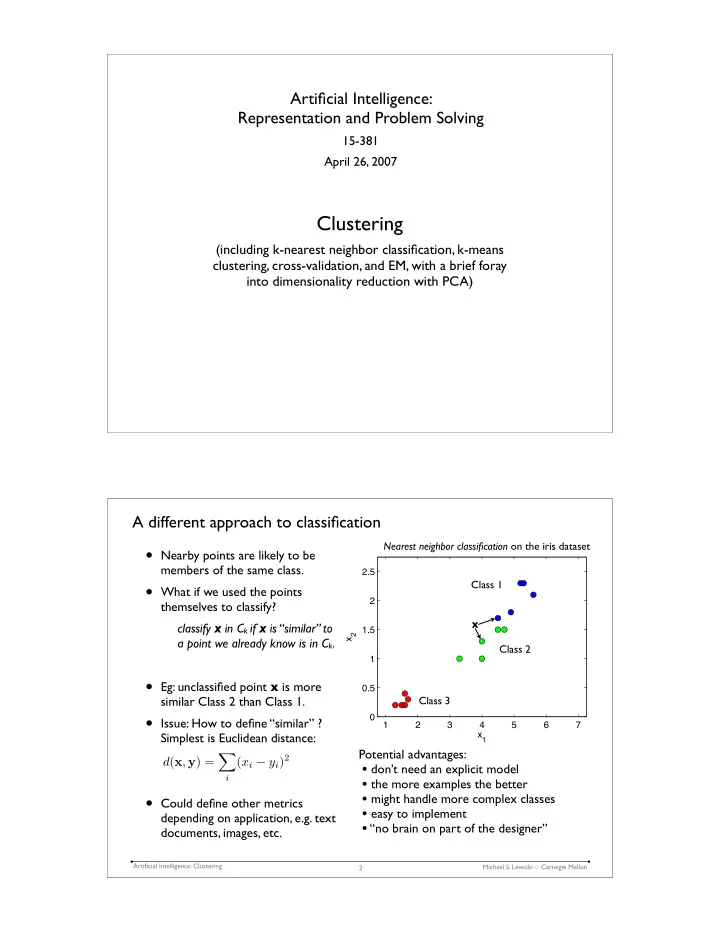
• Nearby points are likely to be

members of the same class.

• What if we used the points

themselves to classify? classify x in Ck if x is “similar” to a point we already know is in Ck.

• Eg: unclassified point x is more

similar Class 2 than Class 1.

• Issue: How to define “similar” ?

Simplest is Euclidean distance:

• Could define other metrics

depending on application, e.g. text documents, images, etc.

1 2 3 4 5 6 7 0.5 1 1.5 2 2.5 x1 x2

x Class 1 Class 2 Class 3

Potential advantages:

• don’t need an explicit model
• the more examples the better
• might handle more complex classes
• easy to implement
• “no brain on part of the designer”

Nearest neighbor classification on the iris dataset

d(x, y) =

• i

(xi − yi)2

Michael S. Lewicki Carnegie Mellon Artificial Intelligence: Clustering

A complex, non-parametric decision boundary

• How do we control the complexity
• f this model?
• difficult
• How many parameters?
• every data point is a parameter!
• This is an example of a non-parametric

model, ie where the model is defined by the data. (Also, called, instance based)

• Can get very complex decision

boundaries

3 example from Martial Herbert Michael S. Lewicki Carnegie Mellon Artificial Intelligence: Clustering

Example: Handwritten digits

• Use Euclidean distance to see which

known digit is closest to each class.

• But not all neighbors are the same:
• “k-nearest neighbors”:

look at k-nearest neighbors and choose most frequent.

• Cautions: can get expensive to find

neighbors

4 from LeCun etal, 1998 digit data available at: http://yann.lecun.com/exdb/mnist/

example nearest neighbors

example from Sam Roweis

Digits are just represented as a vector.

Michael S. Lewicki Carnegie Mellon Artificial Intelligence: Clustering

The problem of using templates (ie Euclidean distance)

• Which of these is more like the

example? A or B?

• Euclidean distance only cares about

how many pixels overlap.

• Could try to define a distance metric

that is insensitive to small deviations in position, scale, rotation, etc.

• Digit example:
• 60,000 training images,
• 10,000 test images
• no “preprocessing”

5

example A B

from Simard etal, 1998

Classifier error rate on test data (%) linear 12.0 k=3 nearest neighbor (Euclidean distance) 5.0 2-layer neural network (300 hidden units) 4.7 nearest neighbor (Euclidean distance) 3.1 k-nearest neighbor (improved distance metric) 1.1 convolutional neural net 0.95 best (the conv. net with elastic distortions) 0.4 humans 0.2 - 2.5 performance results of various classifiers (from http://yann.lecun.com/exdb/mnist/)

Clustering

Michael S. Lewicki Carnegie Mellon Artificial Intelligence: Clustering

Clustering: Classification without labels:

7

• In many situations we don’t have labeled training data, only unlabeled data.
• Eg, in the iris data set, what if we were just starting and didn’t know any classes?

1 2 3 4 5 6 7 0.5 1 1.5 2 2.5 petal length (cm) petal width (cm)

Michael S. Lewicki Carnegie Mellon Artificial Intelligence: Clustering

Types of learning

8

world (or data) model {θ1, . . . , θn} desired output {y1, . . . , yn} supervised world (or data) model {θ1, . . . , θn} unsupervised world (or data) model {θ1, . . . , θn} model output reinforcement reinforcement next week

Michael S. Lewicki Carnegie Mellon Artificial Intelligence: Clustering

A real example: clustering electrical signals from neurons

• scilloscope

software analysis electrode filters amplifier A/D

9

Basic problem: only information is signal. The true classes are always unknown.

Michael S. Lewicki Carnegie Mellon Artificial Intelligence: Clustering

An extracellular waveform with many different neural “spikes”

5 10 15 20 25 msec

How do we sort the different spikes?

10

Michael S. Lewicki Carnegie Mellon Artificial Intelligence: Clustering

Sorting with level detection

11

0.5 0.5 1 1.5 msec 0.5 0.5 1 1.5 msec

Level detection doesn’t always work.

Michael S. Lewicki Carnegie Mellon Artificial Intelligence: Clustering

Why level detection doesn’t work

12

background amplitude

A B

amplitude peak amplitude: neuron 2 peak amplitude: neuron 1

One dimension is not sufficient to separate the spikes.

0.5 0.5 1 1.5 msec 0.5 0.5 1 1.5 msec

Michael S. Lewicki Carnegie Mellon Artificial Intelligence: Clustering

Idea: try more features

13

0.5 0.5 1 1.5 msec

What other features could we use?

max amplitude min amplitude

Michael S. Lewicki Carnegie Mellon Artificial Intelligence: Clustering

Maximum vs minimum

14

200 150 100 50 50 100 150 200 250 spike minimum (µV) spike maximum (µV)

This allows better discrimination than max alone, but is it optimal?

Michael S. Lewicki Carnegie Mellon Artificial Intelligence: Clustering

Try different features

15

0.5 0.5 1 1.5 msec

What other features could we use?

height width

Michael S. Lewicki Carnegie Mellon Artificial Intelligence: Clustering

Height vs width

16

0.5 1 1.5 50 100 150 200 250 300 350 400 spike width (msec) spike height (µV)

This allows allows better discrimination. How can we choose more objectively?

Brief foray: dimensionality reduction (in this modeling data with a normal distribution)

Michael S. Lewicki Carnegie Mellon Artificial Intelligence: Clustering

• Idea: model the distribution of the data.

This is density estimation

• We’ve done this before:
• Bernoulli distribution of coin flips:
• Gaussian distribution of iris data:

1 2 3 4 5 6 7 18

data (neural signals) model {θ1, . . . , θn}

Can we model the signal with a better set of features?

unsupervised learning

p(y|θ, n) = n y

• θy(1 − θ)n−y

1 2 3 4 5 6 7 0.5 1 1.5 2 2.5 petal length (cm) petal width (cm)

p(x|µ, σ) = 1 √ 2πσ exp

• − 1

2σ2 (x − µ)2

Michael S. Lewicki Carnegie Mellon Artificial Intelligence: Clustering

“Modeling” data with a Gaussian

• a Gaussian (or normal) distribution is “fit” to data with things you’re already

familiar with.

• A multivariate normal is the same but in d-dimensions

19

µ = 1 N

• n

xn σ2 = 1 N

• n

(xn − µ)2 p(x|µ, σ) = 1 √ 2πσ exp

• − 1

2σ2 (x − µ)2

• mean

variance

N (µ, Σ) = (2π)−d/2|Σ|−1/2 exp

• −1

2(x − µ)T Σ−1(x − µ)

• ˆ

µ = 1 N

• n

xn ˆ Σij = 1 N − 1

• n

(xi,n − ˆ µ)(xj,n − ˆ µ)

Michael S. Lewicki Carnegie Mellon Artificial Intelligence: Clustering

#$C;'(;2D4,E2+F(+($2

GHI%)054()*+J,K L.M7N0.O//P

!

"#$ !

" !

"#$ !

" %&&

'()$*+ !

" %&&

'()$*+ !

"

20

Recall the example from the probability theory lecture

Michael S. Lewicki Carnegie Mellon Artificial Intelligence: Clustering

#$C;'(;2D4,E2+F(+($2

GHI%)054()*+J,K L.M7N0.O//P

!

"#$ !

" !

"#$ !

" %&&

'()$*+ !

" %&&

'()$*+ !

"

9'(2D(%;< G()42C4D+$' $R,#

21

What about distributions in higher dimensions?

The correlational structure is described by the covariance

Michael S. Lewicki Carnegie Mellon Artificial Intelligence: Clustering 22

Multivariate covariance matrices and principal components

Head measurements on two college-age groups (Bryce and Barker): 1) football players (30 subjects) 2) non-football players (30 subjects) Use six different measurements: variable measurement WDMI head width at widest dimention CIRCUM head circumference FBEYE front to back at eye level EYEHD eye to top of head EARHD ear to top of head JAW jaw width Are these measures independent?

Michael S. Lewicki Carnegie Mellon Artificial Intelligence: Clustering

The covariance matrix

S =         .370 .602 .149 .044 .107 .209 .602 2.629 .801 .666 .103 .377 .149 .801 .458 .012 −.013 .120 .044 .666 .011 1.474 .252 −.054 .107 .103 −.013 .252 .488 −.036 .209 .377 .120 −.054 −.036 .324         Sij = 1 N − 1

N

• n=1

(xi,n − ¯ xi)(xj,n − ¯ xj)

23 Michael S. Lewicki Carnegie Mellon Artificial Intelligence: Clustering

The eigenvalues

Proportion Cumulative Eigenvalue

• f Variance

Proportion 3.323 .579 .579 1.374 .239 .818 .476 .083 .901 .325 .057 .957 .157 .027 .985 .088 .015 1.000 How many PCs should we select?

24

Michael S. Lewicki Carnegie Mellon Artificial Intelligence: Clustering

The eigenvalues

Proportion Cumulative Eigenvalue

• f Variance

Proportion 3.323 .579 .579 1.374 .239 .818 .476 .083 .901 .325 .057 .957 .157 .027 .985 .088 .015 1.000 How many PCs should we select? The first two principal components capture 81.8% of the variance.

25 Michael S. Lewicki Carnegie Mellon Artificial Intelligence: Clustering

The eigenvalues

Proportion Cumulative Eigenvalue

• f Variance

Proportion 3.323 .579 .579 1.374 .239 .818 .476 .083 .901 .325 .057 .957 .157 .027 .985 .088 .015 1.000 How many PCs should we select? The first two principal components capture 81.8% of the variance.

26

The corresponding eigenvectors: variable a1 a2 WDMI .207

• .142

CIRCUM .873

• .219

FBEYE .261

• .231

EYEHD .326 .891 EARHD .066 .222 JAW .128

• .187

Michael S. Lewicki Carnegie Mellon Artificial Intelligence: Clustering

Using principal components to characterize the data

27

• What are the data?

ata?

0.5 0.5 1 150 100 50 50 100 150 200 msec amplitude (µV)

What is the dimensionality of the data? How many components are there? What will the components look like?

Michael S. Lewicki Carnegie Mellon Artificial Intelligence: Clustering

The first three principal components of the waveform data

28

0.5 0.5 1 0.3 0.2 0.1 0.1 0.2 0.3 0.4 msec magnitude PC1 PC2 PC3

What do you expect when we plot PC1 vs PC2 ?

Michael S. Lewicki Carnegie Mellon Artificial Intelligence: Clustering

Scatter plot of the first two principal component scores

29

200 200 400 600 400 300 200 100 100 200 300 400 1st component score 2nd component score

Now the data are much better separated. Could we use more PCs? How many?

Michael S. Lewicki Carnegie Mellon Artificial Intelligence: Clustering

The eigenspectrum of the waveform data

30

10 20 30 40 50 20 40 60 80 100 component number sqrt() (µV)

Michael S. Lewicki Carnegie Mellon Artificial Intelligence: Clustering

Recall example from last lecture: waveform data

31

• The waveform x is modeled with a

multivariate Gaussian x ∼ p(x|µ, Σ)

• µ and Σ are mean and covariance of

the distribution.

• Principal components can be used to

form a low-dimensional approximation x(n) =

T

• i=1

c(n)

i

φi

• The vectors {φ1, . . . , φT} are the

eigenvectors of Σ.

• keeping on the first two terms in the

sum is an adequate approximation of the full T-dimensional density.

!!"# ! !"# $ !$#! !$!! !#! ! #! $!! $#! %!! &'() *&+,-./0(12µ34

raw spike waveform data

!"# !"$ !"%

now we can go back to clustering

Michael S. Lewicki Carnegie Mellon Artificial Intelligence: Clustering

Now try clustering our 2d data (could also do it in n-d)

!!"" " !"" #"" $"" !#"" !!"" " !"" #"" $"" !%&'()'%*+,- #./'()'%*+,-

33 Michael S. Lewicki Carnegie Mellon Artificial Intelligence: Clustering

k-means clustering

34

• Idea: try to estimate k cluster centers by

minimizing “distortion”

• Define distortion as:
• rnk is 1 for the closest cluster mean to xn.
• Each point xn is the minimum distance

from its closet center.

• How do we learn the cluster means?
• Use EM = Estimate Maximize

D =

N

• n=1

K

• k=1

rnk xn − µk 2 rnk = 1 if xn ∈ cluster k, 0 otherwise.

Michael S. Lewicki Carnegie Mellon Artificial Intelligence: Clustering

Using EM to estimate the cluster means

• Our objective function is:
• Differential wrt to the mean (the

parameter we want to estimate):

• We know the optimum is when
• Solving for the mean we have:
• This is simply a weighted mean for

each cluster.

• Thus we have a simple estimation

algorithm (k-means clustering)

• 1. select k points at random
• 2. estimate (update) means
• 3. repeat until converged
• convergence (to a local minimum) is

guaranteed

35

D =

N

• n=1

K

• k=1

rnk xn − µk 2 ∂D ∂µk = 2

N

• n=1

rnk(xn − µk) ∂D ∂µk = 2

N

• n=1

rnk(xn − µk) = 0 µk =

• n rnkxn
• n rnk

Michael S. Lewicki Carnegie Mellon Artificial Intelligence: Clustering

k-means clustering example

!!"" " !"" #"" $"" !#"" !!"" " !"" #"" $"" !%&'()'%*+,- #./'()'%*+,-

36

Select 3 points at random for cluster means

Michael S. Lewicki Carnegie Mellon Artificial Intelligence: Clustering

!!"" " !"" #"" $"" !#"" !!"" " !"" #"" $"" !%&'()'%*+,- #./'()'%*+,-

k-means clustering example

!!"" " !"" #"" $"" !#"" !!"" " !"" #"" $"" !%&'()'%*+,- #./'()'%*+,-

37

The update them using the estimate.

Michael S. Lewicki Carnegie Mellon Artificial Intelligence: Clustering

k-means clustering example

!!"" " !"" #"" $"" !#"" !!"" " !"" #"" $"" !%&'()'%*+,- #./'()'%*+,-

38

And iterate...

Michael S. Lewicki Carnegie Mellon Artificial Intelligence: Clustering

k-means clustering example

!!"" " !"" #"" $"" !#"" !!"" " !"" #"" $"" !%&'()'%*+,- #./'()'%*+,-

39 Michael S. Lewicki Carnegie Mellon Artificial Intelligence: Clustering

k-means clustering example

!!"" " !"" #"" $"" !#"" !!"" " !"" #"" $"" !%&'()'%*+,- #./'()'%*+,-

40

Stop when converged, ie no change.

Michael S. Lewicki Carnegie Mellon Artificial Intelligence: Clustering

An example of a local minimum

! "!! #!! $!! !"!! !#!! !"!! ! "!! #!! $!! "%&'()'%*+,- #./'()'%*+,-

41

There can be multiple local minima.

Michael S. Lewicki Carnegie Mellon Artificial Intelligence: Clustering 1 2 3 4 5 6 7 8 9 10 1 2 3 4 5 6 7 8 9 10 k = number of clusters Distortion

How do we choose k?

42

• Increasing k, will always decrease our

distortion, so we will overfit.

• How can we avoid this?
• Or how do we choose the best k?
• We can use cross validation again.
• Instead of classification error,

however, like before, we use our distortion metric:

• Then just measure the distortion on

a test data set, and stop when we reach a minimum. D =

N

• n=1

K

• k=1

rnk xn − µk 2

!!"" " !"" #"" $"" !#"" !!"" " !"" #"" $"" !%&'()'%*+,- #./'()'%*+,-

k=10 clusters

• verfitting

Michael S. Lewicki Carnegie Mellon Artificial Intelligence: Clustering 43

Example

• Construct a predictor of y from x given this

training data x y A nice illustration of cross validation from Andrew Moore

Michael S. Lewicki Carnegie Mellon Artificial Intelligence: Clustering

x y x y x y Linear Quadratic Piecewise Linear Which model is best for predicting y from x ????

44

Michael S. Lewicki Carnegie Mellon Artificial Intelligence: Clustering

x y x y x y Linear Quadratic Piecewise Linear Which model is best for predicting y from x ???? We want the model that generate the best predictions on future data. Not necessarily the one with the lowest error on training data

45 Michael S. Lewicki Carnegie Mellon Artificial Intelligence: Clustering

Using a Test Set

• 1. Use a portion

(e.g., 30%) of the data as test data

• 2. Fit a model to

the remaining training data

• 3. Evaluate the

error on the test data x y

46

Michael S. Lewicki Carnegie Mellon Artificial Intelligence: Clustering

x y x y x y Linear Quadratic Error = 2.4 Error = 2.2 Error = 0.9 Piecewise Linear

47 Michael S. Lewicki Carnegie Mellon Artificial Intelligence: Clustering

x y x y x y Linear Quadratic Error = 2.4 Error = 2.2 Error = 0.9 Piecewise Linear Using a Test Set: + Simple

• Wastes a large % of the data
• May get lucky with one

particular subset of the data

48

Michael S. Lewicki Carnegie Mellon Artificial Intelligence: Clustering

“Leave One Out” Cross-Validation

• For k=1 to R

– Train on all the data leaving out (xk,yk) – Evaluate error

• n (xk,yk)
• Report the

average error after trying all the data points

x y

(xk,yk)

49 Michael S. Lewicki Carnegie Mellon Artificial Intelligence: Clustering

Error = 2.12

Note: Numerical examples in this and subsequent slides from A. Moore

50

Michael S. Lewicki Carnegie Mellon Artificial Intelligence: Clustering

Error = 0.962

51 Michael S. Lewicki Carnegie Mellon Artificial Intelligence: Clustering

Error = 3.33

52

Michael S. Lewicki Carnegie Mellon Artificial Intelligence: Clustering

Leave One Out Cross-Validation

• For k=1 to R

– Train on all the data leaving out (xk,yk) – Evaluate error

• n (xk,yk)
• Report the

average error after trying all the data points

x y

(xk,yk)

“Leave One Out” Cross-Validation: + Does not waste data + Average over large number of trials

• Expensive

53 Michael S. Lewicki Carnegie Mellon Artificial Intelligence: Clustering

K-Fold Cross-Validation

• Randomly divide

the data set into K subsets

• For each subset

S:

– Train on the data not in S – Test on the data in S

• Return the

average error over the K subsets x y Example: K = 3, each color corresponds to a subset

54

Michael S. Lewicki Carnegie Mellon Artificial Intelligence: Clustering

Error = 2.05 Error = 1.11 Error = 2.93

55 Michael S. Lewicki Carnegie Mellon Artificial Intelligence: Clustering

Cross-Validation Summary

Wastes only 1/K of the data! Only K times slower than Test Set! Wastes 1/K of the data K times slower than Test Set K-Fold Does not waste data Inefficient Leave One Out Simple/Efficient Wastes a lot of data Poor predictor

• f future

performance Test Set

+

• 56

Michael S. Lewicki Carnegie Mellon Artificial Intelligence: Clustering

A probabilistic interpretation: Gaussian mixture models

57

• We’ve already seen a one-dimensional version
• This example has three classes: neuron 1, neuron 2, and background noise.
• Each can be modeled as a Gaussian
• Any given data point comes from just one Gaussian
• The whole set of data is modeled by a mixture of three Gaussians
• How do we model this?

background amplitude

A B

amplitude peak amplitude: neuron 2 peak amplitude: neuron 1

Michael S. Lewicki Carnegie Mellon Artificial Intelligence: Clustering

The Gaussian mixture model density

58

• The likelihood of the data given a particular class ck is given by

p(x|ck, µk, Σk)

• x is the spike waveform, µk and Σk are the mean and covariance for class ck.
• The marginal likelihood is computed by summing over the likelihood of the K classes

p(x|θ1:K) =

K

• k=1

p(x|ck, θk)p(ck)

• θ1:K defines the parameters for all of the classes, θ1:K = {µ1, Σ1, . . . , µK, ΣK}.
• p(ck) is the probability of the kth class, with

k p(ck) = 1.

• What does this mean in this example?

Michael S. Lewicki Carnegie Mellon Artificial Intelligence: Clustering

• How do we determine the class ck from the data x ?
• Again use Bayes’ rule

p(ck|x(n), θ1:K) = pk,n = p(x(n)|ck, θk)p(ck)

• k p(x(n)|ck, θk)p(ck)
• This tells is the probability that waveform x(n) came from class ck.

Bayesian classification

59

• Let’s review the process:

1. define model of problem 2. derive posterior distributions and estimators 3. estimate parameters from data ?? 4. evaluate model accuracy How do we do this?

Michael S. Lewicki Carnegie Mellon Artificial Intelligence: Clustering

Estimating the parameters: fitting the model density to the data

• The objective of density estimation is to maximize the likelihood of the data the data
• If we assume the samples are independent, the data likelihood is just the product of

the marginal likelihoods p(x1:N|θ1:K) =

N

• n=1

p(xn|θ1:K)

• The class parameters are determined by optimization.
• Is far more practical to optimize the log-likelihood.
• One elegant approach to this is the EM algorithm.

60

Michael S. Lewicki Carnegie Mellon Artificial Intelligence: Clustering

The EM algorithm

• EM stands for Expectation-Maximization, and involves two steps that are iterated.

For the case of a Gaussian mixture model:

• 1. E-step: Compute pn,k = p(ck|x(n), θ1:K). Let pk =

n pi,n

• 2. M-step: Compute new mean, covariance, and class prior for each class:

µk ←

• n

pn,kx(n)/pk Σk ←

• n

pn,k(x(n) − µk)(x(n) − µk)T/pk p(ck) ← pk

• This is just the sample mean and covariance, weighted by the class conditional

probabilities pn,k.

• Derived by solving setting log-likelihood gradient to zero (i.e. the maximum).

61

Something can go bad here... What if these are zero?

Michael S. Lewicki Carnegie Mellon Artificial Intelligence: Clustering

Four cluster solution with decision boundaries

62

!!"" " !"" #"" $"" !#"" !%"" !!"" !&"" " &"" !"" %"" #"" &'()*+,-+./.()'*+0/ !.1)*+,-+./.()'*+0/

Michael S. Lewicki Carnegie Mellon Artificial Intelligence: Clustering

But wait! Here’s a nine cluster solution

63

200 200 400 600 400 300 200 100 100 200 300 400 1st component score 2nd component score

Uh oh... How many clusters are there really? Fortunately, probability theory solves this problem too.

Michael S. Lewicki Carnegie Mellon Artificial Intelligence: Clustering

Bayesian model comparison

64

• Let MK represents a model with K classes. (Here we will assume that we can

choose the best among all such models, but this assumption is not necessary). How do we evaluate the probability of model MK? Bayes rule again.

• We start with our existing model, but add a term to represent the model itself. Also,

we marginalize out the dependency on the parameters, because we want the result independent of any specific value. Letting X = x(1:N), we have p(MK|X) = p(X|MK)p(MK) p(X)

• The denominator is constant across models, and if we assume all models are equally

probable a priori, the only data-dependent term is X = x(1:N).

• How do we compute p(X|MK)? We’ve encountered this before.

Michael S. Lewicki Carnegie Mellon Artificial Intelligence: Clustering

Evaluating the model evidence

• p(X|MK) is just the normalizing constant for the posterior for parameters

p(θK|X, MK) = p(X|θK, MK)p(MK) p(X|MK)

• (slight change of notation: θK represents all parameters for model K.)
• The normalizing constant here is evaluated just like before by marginalization

p(X|MK) =

• p(X|θK, MK)p(MK)dθK
• Evaluating this term is practically a whole subfield of probability theory: Laplace’s

method, monte carlo integration, variational approximation, etc. We will learn about some of these techniques in future lectures.

65 Michael S. Lewicki Carnegie Mellon Artificial Intelligence: Clustering

Back to the clusters

66

!!"" " !"" #"" $"" !#"" !%"" !!"" !&"" " &"" !"" %"" #"" &'()*+,-+./.()'*+0/ !.1)*+,-+./.()'*+0/ 200 200 400 600 400 300 200 100 100 200 300 400 1st component score 2nd component score

• Which model is more probable?
• P(M9 | X) is exp(160) times greater than P(M4 | X).
• Why might this not agree with our “intuitions”?
• The conclusions are always only as valid as the model.
• But P(M9 | X) is exp(16) times greater than P(M11 | X).
• This embodies Occam’s Razor.

Michael S. Lewicki Carnegie Mellon Artificial Intelligence: Clustering

Comparison to cross-validation

67

• does not “waste” any data
• correct, if model is correct
• can be expensive or difficult to evaluate for complex models
• harder to implement (definitely “requires a brain”)

Michael S. Lewicki Carnegie Mellon Artificial Intelligence: Clustering

Summary

• k-nearest neighbor: a simple, non-parametric method for classification
• easy to implement, but hard to control the complexity
• can require a lot of data, since there’s no model to generalize from
• clustering:
• is unsupervised learning
• have to infer classes without labels
• dimensionality reduction and PCA
• another example of unsupervised learning: fitting a multivariate normal
• cross validation
• a general way to control complexity: test data, “leave one out”, “k-fold”
• gaussian mixture models
• a probabilistic version of k-means
• can assume arbitrary covariance matrices
• can choose most probable # of clusters (with Bayesian model comparison)

68