A Note on Solution Sizes in the Haplotype Tagging SNPs Problem Staal Vinterbo 1 Stephan Dreiseitl 2 1 Decision Systems Groups Harvard Medical School, Boston, USA 2 Dept. of Software Engineering Upper Austria University of Applied Sciences Hagenberg, Austria EMSS 2006, Barcelona, Oct. 5 th 2006
Overview • Biomedical background • Haplotype tagging problem • Approximation algorithm • Solution size investigation
Genomic biology primer Genetic information stored in DNA, ∼ 3 billion base pairs ( homo sapiens )
Genomic biology primer Genetic information stored in DNA, ∼ 3 billion base pairs ( homo sapiens ) Compare with amoeba dubia : ∼ 670 billion base pairs
Genomic biology primer Genetic information stored in DNA, ∼ 3 billion base pairs ( homo sapiens ) Compare with amoeba dubia : ∼ 670 billion base pairs Genes are protein-coding regions, comprise about 3–5% of human genome ( ∼ 25 000 genes)
Genomic biology primer Genetic information stored in DNA, ∼ 3 billion base pairs ( homo sapiens ) Compare with amoeba dubia : ∼ 670 billion base pairs Genes are protein-coding regions, comprise about 3–5% of human genome ( ∼ 25 000 genes) Compare with oryza sativa : ∼ 40 000–60 000 genes
Genomic biology primer DNA of individual humans is 99.9% identical
Genomic biology primer DNA of individual humans is 99.9% identical Sequence variations:
Genomic biology primer Single nucleotide polymorphism (SNP): Small genetic variation in a person’s DNA sequence T A A C T A A C T A A A T A A C ↑ SNP
Genomic biology primer Single nucleotide polymorphism (SNP): Small genetic variation in a person’s DNA sequence T A A C T A A C T A A A T A A C ↑ SNP Consider only variations occuring in > 1% of population About 10 million SNPs currently known
Effects of sequence variations
Effects of sequence variations
Effects of sequence variations
Effects of sequence variations
Genomic biology primer SNPs in close proximity are not independent ( linkage disequilibrium )
Genomic biology primer SNPs in close proximity are not independent ( linkage disequilibrium ) Haplotype: Set of associated SNPs in a region of a chromosome T A A C T A A C C T A A C A A T T T A A A C A A A T A C A C A A
Genomic biology primer SNPs in close proximity are not independent ( linkage disequilibrium ) Haplotype: Set of associated SNPs in a region of a chromosome T A A C T A A C C T A A C A A T T T A A A C A A A T A C A C A A Haplotype-tagging SNPs (htSNPs): Those SNPs that allow the unique identification of a haplotype
Genomic biology primer SNPs in close proximity are not independent ( linkage disequilibrium ) Haplotype: Set of associated SNPs in a region of a chromosome T A A C T A A C C T A A C A A T T T A A A C A A A T A C A C A A ↑ ↑ Haplotype-tagging SNPs (htSNPs): Those SNPs that allow the unique identification of a haplotype
Medical significance Diseases caused by variations in single genes are rare
Medical significance Diseases caused by variations in single genes are rare Common disorders are caused by combined effect of different variants and environmental influences
Medical significance Diseases caused by variations in single genes are rare Common disorders are caused by combined effect of different variants and environmental influences Association studies: Compare haplotype of diseased with that of healthy individuals
Medical significance Diseases caused by variations in single genes are rare Common disorders are caused by combined effect of different variants and environmental influences Association studies: Compare haplotype of diseased with that of healthy individuals Advantages of htSNPs: Only need to test few locations to identify complete haplotype
Medical significance
Problem statement Given: n haplotypes h 1 , . . . , h n with m SNPs each, e.g. h 1 = T A A C T A A C h 2 = C T A A C A A T h 3 = T T A A A C A A h 4 = A T A C A C A A
Problem statement Given: n haplotypes h 1 , . . . , h n with m SNPs each, e.g. h 1 = T A A C T A A C h 2 = C T A A C A A T h 3 = T T A A A C A A h 4 = A T A C A C A A Let h i [ S ] denote values of h i at positions in index set S ⊆ { 1 , . . . , m }
Problem statement Given: n haplotypes h 1 , . . . , h n with m SNPs each, e.g. h 1 = T A A C T A A C h 2 = C T A A C A A T h 3 = T T A A A C A A h 4 = A T A C A C A A Let h i [ S ] denote values of h i at positions in index set S ⊆ { 1 , . . . , m } Find: Minimum cardinality set S s.t. ∀ i , j h i [ S ] = h j [ S ] ⇒ i = j
Problem statement Given: n haplotypes h 1 , . . . , h n with m SNPs each, e.g. h 1 = T A A C T A A C h 2 = C T A A C A A T h 3 = T T A A A C A A h 4 = A T A C A C A A ↑ Let h i [ S ] denote values of h i at positions in index set S ⊆ { 1 , . . . , m } Find: Minimum cardinality set S s.t. ∀ i , j h i [ S ] = h j [ S ] ⇒ i = j
Problem statement Given: n haplotypes h 1 , . . . , h n with m SNPs each, e.g. h 1 = T A A C T A A C h 2 = C T A A C A A T h 3 = T T A A A C A A h 4 = A T A C A C A A ↑ ↑ Let h i [ S ] denote values of h i at positions in index set S ⊆ { 1 , . . . , m } Find: Minimum cardinality set S s.t. ∀ i , j h i [ S ] = h j [ S ] ⇒ i = j
Problem statement Given: n haplotypes h 1 , . . . , h n with m SNPs each, e.g. h 1 = T A A C T A A C h 2 = C T A A C A A T h 3 = T T A A A C A A h 4 = A T A C A C A A ↑ ↑ ↑ Let h i [ S ] denote values of h i at positions in index set S ⊆ { 1 , . . . , m } Find: Minimum cardinality set S s.t. ∀ i , j h i [ S ] = h j [ S ] ⇒ i = j
Problem statement Given: n haplotypes h 1 , . . . , h n with m SNPs each, e.g. h 1 = T A A C T A A C h 2 = C T A A C A A T h 3 = T T A A A C A A h 4 = A T A C A C A A ↑ ↑ Let h i [ S ] denote values of h i at positions in index set S ⊆ { 1 , . . . , m } Find: Minimum cardinality set S s.t. ∀ i , j h i [ S ] = h j [ S ] ⇒ i = j
Problem analysis Minimum haplotype tagging problem is NP-hard via reduction to minimum set cover (MSC) problem MSC problem: Given X = { x 1 , . . . , x n } and set F of subsets of X , find minimum cardinality C ⊆ F s.t. � c ∈ C c = X
Problem analysis Minimum haplotype tagging problem is NP-hard via reduction to minimum set cover (MSC) problem MSC problem: Given X = { x 1 , . . . , x n } and set F of subsets of X , find minimum cardinality C ⊆ F s.t. � c ∈ C c = X Simple greedy approximation algorithm
Greedy approximation algorithm For data matrix H , let d be discernability function � � d ( i ) := ( j , k ) | H ji � = H ki , j < k Example: T A A C T A A C C T A A C A A T H = T T A A A C A A A T A C A C A A
Greedy approximation algorithm For data matrix H , let d be discernability function � � d ( i ) := ( j , k ) | H ji � = H ki , j < k Example: T A A C T A A C C T A A C A A T H = T T A A A C A A A T A C A C A A d (1) = { (1 , 2) , (1 , 4) , (2 , 3) , (2 , 4) , (3 , 4) } d (2) = { (1 , 2) , (1 , 3) , (1 , 4) } d (3) = {}
Greedy approximation algorithm S ← ∅ cols ← { 1 , . . . , m } D ← d (cols) while D � = ∅ select c ∈ cols that maximizes | D ∩ d ( c ) | D ← D \ d ( c ) S ← S ∪ { c } return S
Algorithm example T A A C T A A C C T A A C A A T T T A A A C A A A T A C A C A A
Algorithm example T A A C T A A C C T A A C A A T T T A A A C A A A T A C A C A A (1 , 2) (1 , 2) (1 , 2) (1 , 2) (1 , 3) (1 , 2) (1 , 4) (1 , 3) (1 , 3) (1 , 3) (1 , 4) (1 , 3) (2 , 3) (1 , 4) (2 , 4) (1 , 4) (2 , 3) (1 , 4) (2 , 4) (3 , 4) (2 , 3) (2 , 4) (2 , 3) (3 , 4) (2 , 4) (2 , 4)
Algorithm example T A A C T A A C C T A A C A A T T T A A A C A A A T A C A C A A (1 , 2) (1 , 2) (1 , 2) (1 , 2) (1 , 3) (1 , 2) (1 , 4) (1 , 3) (1 , 3) (1 , 3) (1 , 4) (1 , 3) (2 , 3) (1 , 4) (2 , 4) (1 , 4) (2 , 3) (1 , 4) (2 , 4) (3 , 4) (2 , 3) (2 , 4) (2 , 3) (3 , 4) (2 , 4) (2 , 4) D ← { (1 , 2) , (1 , 3) , (1 , 4) , (2 , 3) , (2 , 4) , (3 , 4) } ; S ← ∅
Algorithm example T A A C T A A C C T A A C A A T T T A A A C A A A T A C A C A A (1 , 2) (1 , 2) (1 , 2) (1 , 2) (1 , 3) (1 , 2) (1 , 4) (1 , 3) (1 , 3) (1 , 3) (1 , 4) (1 , 3) (2 , 3) (1 , 4) (2 , 4) (1 , 4) (2 , 3) (1 , 4) (2 , 4) (3 , 4) (2 , 3) (2 , 4) (2 , 3) (3 , 4) (2 , 4) (2 , 4) D ← { (1 , 2) , (1 , 3) , (1 , 4) , (2 , 3) , (2 , 4) , (3 , 4) } ; S ← ∅ Algorithm step 1: Pick c = 1, 5 or 8 (say 1) D ← D \ d (1) = { 1 , 3 } S ← S ∪ { 1 } = { 1 }
Algorithm example T A A C T A A C C T A A C A A T T T A A A C A A A T A C A C A A (1 , 2) (1 , 2) (1 , 2) (1 , 2) (1 , 3) (1 , 2) (1 , 4) (1 , 3) (1 , 3) (1 , 3) (1 , 4) (1 , 3) (2 , 3) (1 , 4) (2 , 4) (1 , 4) (2 , 3) (1 , 4) (2 , 4) (3 , 4) (2 , 3) (2 , 4) (2 , 3) (3 , 4) (2 , 4) (2 , 4) D = { (1 , 3) } ; S = { 1 }
Recommend
More recommend
Unleash a World of Digital Possibilities—Browse, Share, and Explore Content Without Boundaries