
SLIDE 1
1 Consider two loci and 1 generation of random mating: Random - - PDF document
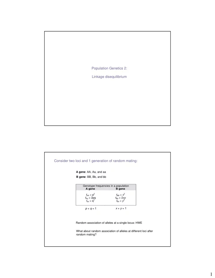
Population Genetics 2: Linkage disequilibrium Consider two loci and 1 generation of random mating: A gene : AA, Aa, and aa B gene : BB, Bb, and bb Genotype frequencies in a population A gene B gene f AA = p 2 f BB = x 2 f Aa = 2pq f Bb = 2 xy f
Random association in gametes Alleles at A locus A(p) a(q) B (x) AB (px) aB (qx) Alleles at B locus b (y) Ab (py) ab (qy) remember: p + q =1 and x + y = 1
Population 1: 100% AABB Population 2: 100% aabb Mix populations equally: 50% AABB + 50% aabb 1 generation of random mating (only three matings possible) : AABB x AABB = AABB aabb x aabb = aabb AABB x aabb = AaBb Nine genotypes are possible: They did not reach equilibrium after one generation of random mating. With continued random mating the “missing” genotypes would appear, but not immediately at their equilibrium frequencies!
AaBB aaBB aaBb AABb AAbb Aabb AABB aabb AaBa
Case 1: AB gamete + ab gamete = AaBb Case 2: Ab gamete + aB gamete = AaBb New symbolism: AB/ab indicates the union of AB gamete + ab gamete
A B a b Physical linkage: Notation = AB/ab
A B a b Physical linkage: Notation = AB/ab
From: iGenetics
page 350
A a Un linked genes: B b
Random association in gametes Alleles at A locus A(p) a(q) B (x) AB (px) aB (qx) Alleles at B locus b (y) Ab (py) ab (qy) remember: p + q =1 and x + y = 1
ts recombinan ts recombinan from random at B and A together putting
prob recomb
prob ts recombinan
generation last in gametes AB
frequency AB ion recombinat no
y probabilit ' AB
AB ' AB
AB
Non-recombinants Recombinants
fs = y = 0.6920 fS = x = 0.3080 Ss blood group fN = q = 0.4575 fM = p = 0.5425 MN blood group Ns = 773/2000 = 0.3865 NS = 142/2000 = 0.0710 Ms = 611/2000 = 0.3055 MS = 474/2000 = 0.2370 Gamete frequencies
max
t recombinan aB Ab t recombinan non aa AB
SS = 483 Ss = 418 ss = 99 MM = 298 MN = 489 NN = 213 Ss locus MN locus
Genotype counts in the population
Ns = 773 NS = 142 Ms = 611 MS = 474 Gametes
Rate of decay of LD under various recombination rates
0.1 0.2 0.3 0.4 0.5 0.6 0.7 0.8 0.9 1 1 9 17 25 33 41 49 57 65 73 81 89 97
generations Standardized disequilibrium D/Dmax r= 0.001 r= 0.01 r= 0.1 r= 0.5
“Hitchhiking” of a mutator gene with and without recombination
Adapted from Sniegowski et al. (2000) BioEssays 22:1057-1066.
No recombination Recombination Mutator allele that increase the mutation rate Beneficial allele subject to strong positive selection
the two genes are physically linked or not.