A A 1 c 1 2 1 If ; ; K ; K 1 2 1 2 c c - PowerPoint PPT Presentation

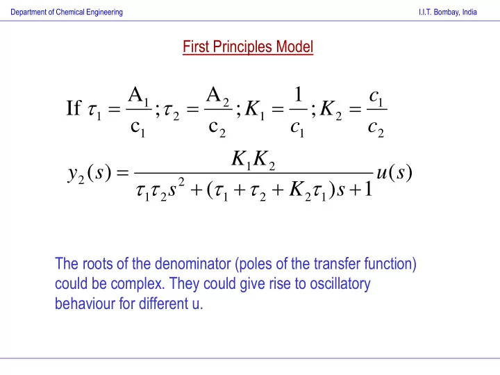
Department of Chemical Engineering I.I.T. Bombay, India First Principles Model A A 1 c       1 2 1 If ; ; K ; K 1 2 1 2 c c c c 1 2 1 2 K K  1 2 y ( s ) u ( s )          2 2 s ( K ) s 1 1 2 1 2 2 1 The roots of the denominator (poles of the transfer function) could be complex. They could give rise to oscillatory behaviour for different u.

Department of Chemical Engineering I.I.T. Bombay, India Second Illustrative example: Control of a first order process + y d y Plant controller u -   t 1  dy     and      u ( t ) K ( y y ) ( y y ) dt y Ku  c d d   dt I 0   t dy 1        Therefore,   y KK ( y y ) ( y y ) dt  c d d dt   I 0 2 d y dy KK      c ( 1 KK ) y y  1 c d 2 dt dt I This is a second order system and will give rise to a second order transfer function.

Department of Chemical Engineering I.I.T. Bombay, India U-Tube Manometer  2 L d h 4 L dh 1    D P 1 P 2 h P   2 2 2 g dt g R dt 2 g L = length of fluid in the plane of h manometer tube initial rest h when D P = 0 ,  = density and viscosity of manometer fluid R = radius of manometer tube D P = P 1 - P 2 g = gravitation constant

Department of Chemical Engineering I.I.T. Bombay, India General second order transfer function For the manometer y ( s ) K     G ( s )       2 2 L 2 6 L u ( s ) s 2 s 1      2 g 3 R g The value of  (damping factor) determines the dynamic response of second order systems. It represents viscous or dissipative forces. If 0   < 1 (underdamped system) - oscillatory approach to steady state  1 (critically damped, overdamped systems) - non-oscillatory approach to steady state.  is also called the natural time constant of the system.

Department of Chemical Engineering I.I.T. Bombay, India Step Response of Overdamped Second Order Systems          t / t / e e A 1 2    1 2   y ( t ) KA 1 u ( s )      s 1 2        t / t / dy e e 1 2    KA      dt 1 2 = 0 at t= 0 Initial Slope = 0. This is in contrast to that of a first order system

Department of Chemical Engineering I.I.T. Bombay, India Step Response of Critically Damped Second Order Systems      A t        t / u ( s ) y ( t ) KA  1 1 e       s     t / dy t e    KA  2   dt = 0 at t= 0 Again, the initial Slope = 0

Department of Chemical Engineering I.I.T. Bombay, India Step Response of Underdamped Second Order Systems                    A 2 2 1 1           t /      u ( s ) y ( t ) KA 1 e cos t sin t             2     1 s             2 1      t /   e sin t          dy    KA    dt  2  1       = 0 at t= 0 Again, the initial Slope = 0

Department of Chemical Engineering I.I.T. Bombay, India Step Response of Underdamped Second Order Systems       1 t ( cos ) r   2 1 Rise time t r : Time at which the output first hits the steady state value t r

Department of Chemical Engineering I.I.T. Bombay, India Peak time Time to first peak t p : Time at which the output hits the first maximum value t p

Department of Chemical Engineering I.I.T. Bombay, India a = max(y) - D y b = D y a Overshoot (OS) = a / b b     OS exp( )   2 1

Department of Chemical Engineering I.I.T. Bombay, India Settling time Time taken to reach and 1.05 * b remain within 5% of the total 0.95 * b change in y (95% response time) b = D y t s

Department of Chemical Engineering I.I.T. Bombay, India a = value of first peak - D y c = value of second peak - D y a c Decay ratio (DR) = c / a      2  OS  2 DR exp( )   2 1

Department of Chemical Engineering I.I.T. Bombay, India Period of Oscillation, P = time between successive peaks = time between successive valleys   2  P   2 1 P         2 1      t /   e sin t          dy    KA    dt  2  1      

Department of Chemical Engineering I.I.T. Bombay, India Frequency Response  y ( s ) K with u ( s ) A sin( wt )     G ( s )      2 2 u ( s ) s 2 s 1 It can be shown that the output y is also a sinusoid with the same frequency as the input and is given by, AK    y ( t ) sin( wt )         t 2 2 2 2 ( 1 w ) ( 2 w ) and     2 w     1 tan     2 2   ( 1 w )