9/7/16 Introduction Pricing and Capacity Provision in Electricity - - PDF document

9/7/16 1

Pricing and Capacity Provision in Electricity Markets An experimental Study

Chloé Le Coq Stockholm School of Economics SITE Henrik Orzen University of Mannheim Sebastian Schwenen Technical University of Munich

Introduction

¤ A problem for market designers: do generators need to be compensated for the provision of peak load electricity? ¤ Basic idea: Compare Energy only and Capacity payments in

terms of their efficiency properties (i.e. ability to efficiently provide capacity) § Do the market rules give the right price signals? § Do the market rules encourage system reliability? § How do price cap levels affects generators’ strategic behavior?

¤ Experimental approach

§ Empirical strategy challenging as counterfactual market outcomes do not exist § Experimental approach: compare different regulatory regimes within a well-defined environment § => virtual electricity market

3

Experimental design, overview

Subjects in the role of firms; 4 firms per market This quadropoly market was played 10 rounds with 6 periods each, (more on timing later) Market interaction: Capacity: up to 9 units q Cost function:

Ø Fixed cost for each unit: 7 Ø Increasing MC: 1 unit costs 1.00; 2 units cost 2.00 etc.

Demand is perfectly price-inelastic but fluctuates

4

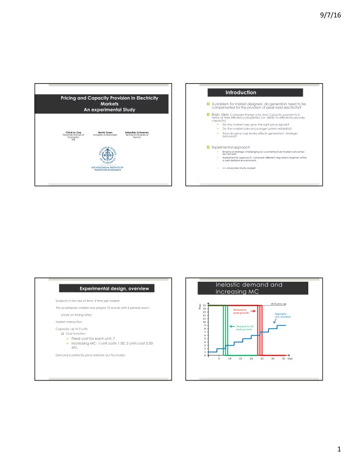
Inelastic demand and increasing MC

• 1

1 2 3 4 5 6 7 8 9 10 11 12 13 14 15 5 10 15 20 25 30 35 Price Unit Aggregate cost schedule Demand in peak periods Demand in off- peak periods e$15 price cap

9/7/16 2

Experimental design, overview (2)

¤ Timing : each round has 6 periods. In each period there is spot market competition with given capacities ¤ Rounds 1 - 2: Each firm has a production capacity of 9 units. ¤ Rounds 3 - 10: Capacities are determined at the beginning of each round. ¤ Treatment variables: ¤ Price cap ¤ Capacity market => 3 treatments Price cap = 15 Price cap = 30 No Capacity market Lowcap HighCap Capacity market Capacity market (CM)

Experimental Design, timing

Uncertain Demand Demand is realized

Stage 1: simultaneous capacity choices (up to 9 units) under demand uncertainty Fixed cost for each unit (=7) + Increasing MC: 1 unit costs 1.00; 2 units cost 2.00 etc. Capacity choices are publicly observed

s = 6

Stage 1 Capacity choices

s = 1 s = 2 s = 3 s = 4 s = 5

Periods

s = 0

Stage 2 Supply function competition (price, quantity)

LOW LOW LOW LOW HIGH HIGH

Stage 1 : Capacity choices

¤ Simultaneously capacity choices under demand uncertainty

Capacity: up to 9 units, Fixed cost for each unit: 7 + Increasing MC: 1 unit costs 1.00; 2 units cost 2.00 etc.

7 ¤ Total Capacity M arket is revealed at the end of the round

Experimental Design, timing

Uncertain Demand Demand is realized

Stage 1: simultaneous capacity choices (up to 9 units) under demand uncertainty Fixed cost for each unit (=7) + Increasing MC: 1 unit costs 1.00; 2 units cost 2.00 etc. Capacity choices are publicly observed Stage 2: price competition for 6 periods with Uniform-price auction

• 1. demand is realized for each period: Low (D=7,8,9) and High (D=23,24,25)
• 2. subjects bid independently and simultaneously: for each unit, bid between 0 and

price cap

s = 6

Stage 1 Capacity choices

s = 1 s = 2 s = 3 s = 4 s = 5

Periods

s = 0

Stage 2 Supply function competition (price, quantity)

LOW LOW LOW LOW HIGH HIGH

9/7/16 3

Stage 2: price choices

¤ The demand is realized, Low (D=6,7,8) and High (D=23,24,25) ¤ For each PERIOD 9 ¤ In addition to the fixed cost of 7, subjects pay a production costs for all units that are dispatched (not for the

• ther units)

¤ Unit 1 (if dispatched), costs 1, the second unit (if dispatched) costs 2, the third unit (if dispatched) costs 3, and so

• n.

¤ The exact number of units that will be dispatched (sold) is revealed in Stage 3.

Experimental Design, timing

Uncertain Demand Demand is realized

Stage 1: simultaneous capacity choices (up to 9 units) under demand uncertainty Fixed cost for each unit (=7) + Increasing MC: 1 unit costs 1.00; 2 units cost 2.00 etc. Capacity choices are publicly observed Stage 2: price competition for 6 periods with Uniform-price auction

• 1. demand is realized for each period: Low (D=7,8,9) and High (D=23,24,25)
• 2. subjects bid independently and simultaneously: for each unit, bid between 0 and price cap

Stage 3. market price equals to highest accepted bid (uniform-price auction)

s = 6

Stage 1 Capacity choices

s = 1 s = 2 s = 3 s = 4 s = 5

Periods

s = 0

Stage 2 Supply function competition (price, quantity)

LOW LOW LOW LOW HIGH HIGH

Stage 3: Market Price and Earnings

¤ M arket supply function: com puter ranks bids from the lowest to the highest ¤ Period’s M arket price: intersection of m arket supply function with inelastic dem and ¤ Screen’s sum m ary of the period 11

Experimental Design, timing for capacity market

Capacity market: Regulator “buys” 25 units of capacity. There is a spot market price cap of 15.00 and a capacity market price cap of 30.00 s = 6

Stage 1a Capacity market

s = 1 s = 2 s = 3 s = 4 s = 5

Periods

s = 0

Stage 2 Supply function competition (price, quantity)

LOW LOW LOW LOW HIGH HIGH

Stage 1b Optional capacity expansion

9/7/16 4

13

Treatments and experimental procedure

Three treatments § Price cap = 15 in LowCap § Price cap = 30 in HighCap § Price cap = 15 and capacity market in CM Experimental procedure : 92 students § Two sessions for each treatment, 3-4 independent markets per session §

• Avg. Payment: $24

14

Theoretical predictions_ Hypotheses

Definition: a pivotal firm j such that 𝐸 − 𝑅$% > 0, where 𝑅$% ≡ ∑ 𝑟+,%

+

and 𝑟% > 0 Hypothesis 1: With at least one pivotal bidder, the equilibrium market price equals the price cap, irrespective of the treatment. Otherwise market price equals the marginal costs of the last dispatched unit Hypotheses 2: Underinvestment in the LowCap treatment and sufficient investment in HighCap and CapMarket are predicted.

Result 1: Avg. Market Capacity over Time

10 15 20 25 30 2 3 4 5 6 7 8 9 10 Average market capacity Round Possible peak demand levels CapMarket HighCap LowCap

=> Towards the end of the experim ent the capacity levels in CAPM ARKET and HIGHCAP are very sim ilar

Result 2: Avg. price over time

=> Intense com petition in off-peak => Peak-periods: Upward trend toward price cap for LowCap and CapM arket BUT not for HighCap => W HY? 5 10 15 20 25 30 1 2 3 4 5 6 7 8 9 10 Price (e$) Round HighCap LowCap CapMarket High price cap: e$30 Low price cap: e$15 Off-peak periods

9/7/16 5

Result 3: price, pivotal bidder, rel. capacity

=> “pivotal” : significant and substantial effect (but not for CapMarket for 8-10 rounds)

Dependent variable: Markup LO WCA P HIG HCA P CA PMA RKET Rounds 1-10 Rounds 8-10 Rounds 1-10 Rounds 8-10 Rounds 1-10 Rounds 8-10 Pivotal 5.800*** (0.000) 7.425*** (0.000) 18.844*** (0.000) 16.417*** (0.009) 2.501*** (0.000) 1.283 (0.277) RelCap (Q-D) 0.009 (0.496) 0.053 (0.246) −0.005 (0.881) −0.145 (0.624) −0.058*** (0.002) −0.164*** (0.003) RelCap × Pivotal −0.095*** (0.007) −0.240*** (0.000) −0.540*** (0.000) −1.013** (0.033) −0.156** (0.040) −0.085 (0.512) Round 0.040 (0.130) −0.016 (0.889) −0.091 (0.170) −1.146** (0.018) 0.035 (0.205) 0.154 (0.361) Number of females −0.272*** (0.000) −0.033 (0.756) −0.346 (0.150) −1.425*** (0.006) −0.185** (0.025) −0.040 (0.790) Constant 0.884** (0.020) −0.179 (0.833) 2.010** (0.039) 8.591 (0.192) 2.000*** (0.000) 3.700*** (0.003) 𝑂 480 144 384 90 480 144 Adjusted 𝑆0 0.741 0.902 0.847 0.808 0.388 0.535

Result 4: treatment effect (rounds 8-10):

HighCap vs. Low Cap (8-10 rounds)

=> High cap treatm ent effect (if pivotal) is due to higher m arket capacity levels

Degree of market power abuse Dependent variable: DMPA = DMPA = 10

0×4$456

4$456 At least one pivotal firm Without pivotal firms HIGHCAP −24.023*** (0.001) −2.941 (0.846) −2.364** (0.044) −3.688 (0.726) CAPMARKET −28.763*** (0.000) −9.714 (0.317) 1.171 (0.342) 44.521*** (0.000) RelCap −3.196** (0.042) 0.257 (0.266) HIGHCAP × RelCap −1.490 (0.680) −0.012 (0.982) CAPMARKET × RelCap −2.651 (0.292) −2.295*** (0.000) Round 3.411 (0.286) 1.560 (0.625) −0.199 (0.708) −0.596 (0.190) Number of females 3.064 (0.295) −0.381 (0.901) −0.874* (0.067) −1.164*** (0.007) Constant 75.927*** (0.000) 85.677*** (0.000) 6.536*** (0.000) 4.209 (0.303) 𝑂 123 123 255 255 Adjusted 𝑆0 0.202 0.271 0.058 0.346

Result 5 : Av. capacity market price

=> Average paid e$ 8.8 in LowCap and e$ 10.3 in CapM arket => Average paid e$ 15.8 in HighCap

1 2 3 4 5 6 7 8 9 10 11 12 13 14 15 3 4 5 6 7 8 9 10 Price (e$) Round 95% confidence interval Mean Marginal capacity cost Equilibrium

Conclusions

¤ Lower spot price and security supply come at the cost of increasing capacity payment ¤ Capacity markets do not rule out market power abuse ¤ Price cap matters for generators’ responsiveness but higher price cap does fully not translate to higher market prices ¤ More treatments: Information available Demand-side bidding Hydropower: subjects are able to save units for the next period

9/7/16 6

Thank you

Chloé Le Coq chloe.lecoq@hhs.se