) ( (6-1) ( = P X ) B f ( x ) dx . X B Note that - PowerPoint PPT Presentation

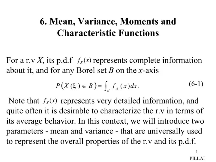
6. Mean, Variance, Moments and Characteristic Functions For a r.v X , its p.d.f represents complete information f X ( x ) about it, and for any Borel set B on the x -axis ) ∫ ( (6-1) ( ξ ∈ = P X ) B f ( x ) dx . X B Note that represents very detailed information, and f X ( x ) quite often it is desirable to characterize the r.v in terms of its average behavior. In this context, we will introduce two parameters - mean and variance - that are universally used to represent the overall properties of the r.v and its p.d.f. 1 PILLAI

Mean or the Expected Value of a r.v X is defined as + ∞ ∫ η = = = (6-2) X E ( X ) x f ( x ) dx . X X − ∞ If X is a discrete-type r.v, then using (3-25) we get ∫ ∑ ∑ ∫ η = = = δ − = δ − X E ( X ) x p ( x x ) dx x p ( x x ) dx X i i i i i � � � � � � � i i 1 ∑ ∑ = = = (6-3) x p x P ( X x ) . i i i i i i Mean represents the average (mean) value of the r.v in a very large number of trials. For example if ∼ then X U ( a , b ), using (3-31) , b 2 2 − 2 + x 1 x b a a b b (6-4) ∫ = = = = E ( X ) dx − − − b a b a 2 2 ( b a ) 2 a a is the midpoint of the interval ( a , b ). 2 PILLAI

On the other hand if X is exponential with parameter as in λ (3-32), then x ∞ ∞ ∫ ∫ − λ − = = λ = λ (6-5) x / y E ( X ) e dx ye dy , λ 0 0 implying that the parameter in (3-32) represents the mean λ value of the exponential r.v. λ Similarly if X is Poisson with parameter as in (3-45), using (6-3), we get λ λ ∞ ∞ k ∞ k ∑ ∑ ∑ = = = − λ = − λ E ( X ) kP ( X k ) ke e k k ! k ! = = = k 0 k 0 k 1 ∞ λ k ∞ λ i ∑ ∑ (6-6) = − λ = λ − λ = λ − λ λ = λ e e e e . − ( k 1 )! i ! = = k 1 i 0 Thus the parameter in (3-45) also represents the mean of λ the Poisson r.v. 3 PILLAI

In a similar manner, if X is binomial as in (3-44), then its mean is given by  n  n n n n ! ∑ ∑ ∑ − − = = =   k n k = k n k E ( X ) kP ( X k ) k p q k p q   − k ( n k )! k !   = = = k 0 k 0 k 1 − − n n ! n 1 ( n 1 )! ∑ ∑ = − = − − = + − = k n k i n i 1 n 1 p q np p q np ( p q ) np . − − − − ( n k )! ( k 1 )! ( n i 1 )! i ! = = k 1 i 0 (6-7) Thus np represents the mean of the binomial r.v in (3-44). For the normal r.v in (3-29), 1 1 + ∞ + ∞ ∫ ∫ 2 2 2 2 − − µ σ − σ = = + µ ( x ) / 2 y / 2 E ( X ) xe dx ( y ) e dy πσ πσ 2 − ∞ 2 − ∞ 2 2 1 1 + ∞ + ∞ ∫ ∫ 2 2 2 2 (6-8) − σ − σ = y / 2 + µ ⋅ y / 2 = µ ye dy e dy . πσ � − ∞ � � � � � � πσ − ∞ 2 2 2 2 � � � � � � � � � 0 1 4 PILLAI

Thus the first parameter in ∼ µ σ is infact the mean of 2 X N ( , ) the Gaussian r.v X . Given ∼ suppose defines a Y = X f ( x ), g ( X ) X new r.v with p.d.f Then from the previous discussion, f Y ( y ). the new r.v Y has a mean given by (see (6-2)) µ Y + ∞ ∫ µ = = E ( Y ) y f ( y ) dy . (6-9) Y Y − ∞ From (6-9), it appears that to determine we need to E ( Y ), determine However this is not the case if only is f Y ( y ). E ( Y ) the quantity of interest. Recall that for any y , ∆ y > 0 ( ) ( ) , ∑ < ≤ + ∆ = < ≤ + ∆ P y Y y y P x X x x (6-10) i i i i where represent the multiple solutions of the equation x i y = g ( x ). But(6-10) can be rewritten as i ∑ (6-11) ∆ = ∆ f ( y ) y f ( x ) x , Y X i i 5 i PILLAI

( ) where the terms form nonoverlapping intervals. + ∆ x , x x i i i Hence ∑ ∑ ∆ = ∆ = ∆ (6-12) y f ( y ) y y f ( x ) x g ( x ) f ( x ) x , Y X i i i X i i i i and hence as ∆ y covers the entire y-axis, the corresponding ∆ x ’s are nonoverlapping, and they cover the entire x -axis. Hence, in the limit as integrating both sides of (6- ∆ y → 0 , 12), we get the useful formula ( ) + ∞ + ∞ ∫ ∫ = = = E ( Y ) E g ( X ) y f ( y ) dy g ( x ) f ( x ) dx . (6-13) Y X − ∞ − ∞ In the discrete case, (6-13) reduces to = ∑ (6-14) = E ( Y ) g ( x ) P ( X x ). i i i From (6-13)-(6-14), is not required to evaluate f Y ( y ) E ( Y ) for We can use (6-14) to determine the mean of Y = g ( X ). Y = where X is a Poisson r.v. Using (3-45) 2 X , 6 PILLAI

( ) ∞ ∞ λ ∞ λ k k ∑ ∑ ∑ = = = − λ = − λ 2 2 2 2 E X k P ( X k ) k e e k k ! k ! = = = k 0 k 0 k 1 + ∞ λ k ∞ λ i 1 ∑ ∑ − − = λ = λ + e k e ( i 1 ) − ( k 1 )! i ! = = k 1 i 0     ∞ λ i ∞ λ i ∞ λ i ∑ ∑ ∑ = λ − λ  +  = λ − λ  + λ  e i e i e     i ! i ! i !     = = = i 0 i 0 i 1     λ λ + ∞ i ∞ m 1 ∑ ∑ − λ  λ  − λ  λ  = λ + = λ + e e e e     − ( i 1 )! m !     = = i 1 m 0 ( ) (6-15) − λ λ λ = λ λ + = λ + λ 2 e e e . ( ) In general, is known as the k th moment of r.v X . k E X Thus if ∼ its second moment is given by (6-15). λ X P ( ) , 7 PILLAI

Mean alone will not be able to truly represent the p.d.f of any r.v. To illustrate this, consider the following scenario: Consider two Gaussian r.vs ∼ and ∼ X N (0,1) X N (0,10). 1 2 Both of them have the same mean However, as µ = 0 . Fig. 6.1 shows, their p.d.fs are quite different. One is more concentrated around the mean, whereas the other one ( X ) 2 has a wider spread. Clearly, we need atleast an additional parameter to measure this spread around the mean! f X 1 x ( ) f X 2 x ( ) 2 1 x x 1 2 2 = 2 = σ σ (b) 10 (a) 1 Fig.6.1 8 PILLAI

For a r.v X with mean represents the deviation of µ − µ , X the r.v from its mean. Since this deviation can be either ( ) , positive or negative, consider the quantity and its 2 − µ X ( ) ] average value represents the average mean − µ 2 E [ X square deviation of X around its mean. Define ( ) ∆ 2 (6-16) σ = − µ > 2 E [ X ] 0 . X With and using (6-13) we get = X − µ 2 g ( X ) ( ) = ∫ + ∞ (6-17) σ − µ > 2 2 ( x ) f ( x ) dx 0 . X − ∞ X σ 2 is known as the variance of the r.v X , and its square X root is known as the standard deviation of σ = − µ 2 E ( X ) X X . Note that the standard deviation represents the root mean square spread of the r.v X around its mean µ . 9 PILLAI

Expanding (6-17) and using the linearity of the integrals, we get ( ) + ∞ ∫ = σ = − µ + µ 2 2 2 Var ( X ) x 2 x f ( x ) dx X X − ∞ + ∞ + ∞ ∫ ∫ = − µ + µ 2 2 x f ( x ) dx 2 x f ( x ) dx X X − ∞ − ∞ ( ) ( ) [ ___ ] 2 2 = − µ = − = − (6-18) 2 2 2 2 E X E X E ( X ) X X . Alternatively, we can use (6-18) to compute σ 2 . X Thus , for example, returning back to the Poisson r.v in (3- 45), using (6-6) and (6-15), we get ___ ( ) (6-19) 2 σ = − = λ + λ − λ = λ 2 2 2 2 X X . X Thus for a Poisson r.v, mean and variance are both equal to its parameter λ . 10 PILLAI

To determine the variance of the normal r.v we µ σ 2 N ( , ), can use (6-16). Thus from (3-29) 1 + ∞ ( ) ∫ 2 2 2 − − µ σ = − µ = − µ 2 ( x ) / 2 Var ( X ) E [( X ) ] x e dx . (6-20) − ∞ πσ 2 2 To simplify (6-20), we can make use of the identity 1 + ∞ + ∞ ∫ ∫ − − µ 2 σ 2 = = ( x ) / 2 f ( x ) dx e dx 1 X πσ − ∞ − ∞ 2 2 for a normal p.d.f. This gives + ∞ ∫ − − 2 2 µ σ = π σ ( x ) / 2 e dx 2 . (6-21) − ∞ σ Differentiating both sides of (6-21) with respect to we , get − µ 2 ( x ) + ∞ ∫ 2 2 − − µ σ ( x ) / 2 = π e dx 2 σ 3 − ∞ or 1 + ∞ ( ) ∫ 2 2 2 − − µ σ (6-22) − µ ( x ) / 2 = σ 2 x e dx , 11 − ∞ πσ 2 2 PILLAI