57% 2. Expose you to lots of new ideas 3. Present a coherent - - PDF document

Statistical Literacy Workshop: Chapter 1 16 May 2019 V1 2019-Schield-USCOTS-Slides1.pdf 1

Chapter 1 by Milo Schield Half-Day Workshop USCOTS May 16, 2019

www.StatLit.org/pdf/2019-Schield-USCOTS-slides1.pdf

Teaching Statistical Literacy

.

First Sharia math, then Sharia law!!!

.

Working Moms; Better Kids

23% more $

Introduction:

• A1. Who takes intro statistics
• A2. SAT level of our students by college
• A3. Math level of our students by major

Exp vs. Obs: What kinds are relevant?

• A3. Kinds of influence on statistics

How common are these influences?

• A4. Grammar: Association vs. causation

Outline

• 1. Present my view of statistical literacy
• 2. Expose you to lots of new ideas
• 3. Present a coherent structure for teaching
• 4. Show the importance of English grammar
• 5. Show simple ways of handling significance
• 6. Show simple ways of handling confounding
• 7. Show how confounding changes significance
• 8. Role-model analyzing studies

Goals of this Workshop

Fraction of 4-year Undergrads that take Intro Stats?

57%

Statistical Literacy Workshop: Chapter 1 16 May 2019 V1 2019-Schield-USCOTS-Slides1.pdf 2

Fraction of Course Gain that Stat Students Loose in 4 Months

50%

Of those taking Stat I:

• less than 1% take Stat II (10-yrs @ U. St. Thomas)
• less than 0.2% major in statistics (nationwide).
• most see less value in statistics after the course than

they did before. Schield and Schield (2008).

• too many say “Worst course I ever took” [anecdotal]

Student Attitudes Toward Stats

What fraction of 4-Yr Intro Stat students are taught outside Math?

50%

Who takes Intro Statistics at Four-Year Colleges?

Where are your students?

SAT Math Scores: Average by Student Major Percentiles

• f all those

taking the Math SAT

SAT Math Percentile by Major

Statistical Literacy Workshop: Chapter 1 16 May 2019 V1 2019-Schield-USCOTS-Slides1.pdf 3

The real world is complex and can't be described well by one or two variables. If students do not have exposure to simple tools for disentangling complex relationships, they may dismiss statistics as an old-school discipline only suitable for small sample inference of randomized studies.

GAISE 2016 Update

Multivariable thinking is critical to make sense of the observational data around us

• learn to identify observational studies
• learn to consider potential confounding factors
• use … stratification … to show confounding

This report recommends that students be introduced to multivariable thinking, preferably early in the introductory course and not as an afterthought at the end of the course.

GAISE 2016 Update

.

Most Important Topics: Student Choices

• *Comparisons: People with degrees earn more than those without

A-B-C Words: A = Association

Causation words assert causation, sufficiency

• r contra-factual

Causation: A bomb caused the fire. Insomnia is a side effect. Lightning resulted in a fire. Spark results in a fire. Sufficient: The more X you do, the more Y you will get. Prevent, stop, end, start, kill, produce, cure, avoid, ban, quit, block, ward off, stave off, cancel, hinder, or eliminate.6 Contra-factual: Those who do X will get more Y than if they had not done X.

A-B-C Words: C = Causation

Between words describe association but imply causation

• *Compare: People who take antidepressants have fewer migraines

A-B-C Words: B = Between

Statistical Literacy Workshop: Chapter 1 16 May 2019 V1 2019-Schield-USCOTS-Slides1.pdf 4

Of the 2,000 news headlines analyzed6, 71% involved A, B or C. Of those headlines involving A, B or C,

• 86% were "between" claims,
• 11% sufficiency, 3% causation, 3% association.
• 6. Schield and Raymond (2009).

A-B-C Words: Distribution in Headlines

This statement is ambiguous. It can mean: 1 Association is not sufficient to prove causation 2 Association provides no evidence for causation. Teachers may intend #1; students often hear #2. A better statement would be: Association is evidence of causation somewhere.

Association is not causation

No idea has stifled the growth of statistical literacy as much as the endless repetition of the words "correlation is not causation". This phrase seems to be primarily used to suppress intellectual inquiry -- by encouraging the unspoken assumption that correlational knowledge is somehow an inferior form of knowledge.

Association is not causation

Studies are the Primary Unit of Analysis

Harvard Case Studies: Title or Abstract

Statistical Literacy : An Overview

Statistical Literacy Workshop: Chapter 1 16 May 2019 V1 2019-Schield-USCOTS-Slides1.pdf 5

Stat Literacy studies Stats as Evidence in Arguments

• Q1. Which group is largest?

Consolidate White (Non-Hispanic) with Hispanic.

• Q2. Which group is largest?

Statistical Literacy : Assembly

Five non-quantitative Topics:

• 1. Regression to the Mean

Sport Illustrated Cover

• 2. Statistically significant
• 3. Chance-Related Mistakes:

Three Door problem; Birthday problem

• Better than chance
• Unlikely to be chance

Statistical Literacy : Randomness

Three kinds of error

• 1. Subject/respondent error:
• 2. Researcher/measurement error:
• 3. Sampling error:

Statistical Literacy : Error/Bias

Statistical Literacy : Assembly

More college students (over half) take intro statistics than any other course (except English). One-size fits all is no longer viable. Statistics education must support Stat 101 and 100/102. Statistics education should (1) support different flavors for different majors, and (2) agree on the contributions of statistics to human knowledge.

Statistical Literacy : Recommendation

Statistical Literacy Workshop: Chapter 1 16 May 2019 V1 2019-Schield-USCOTS-Slides1.pdf 6

The past success of statistics has depended on vast, deliberate simplifications amounting to willful ignorance. This very success now threatens future advances in medicine, the social sciences, and other fields. Limitations of existing methods result in frequent reversals of scientific findings/recommendations, to the consternation of scientists and the public. Herbert I. Weisberg

Willful Ignorance

The past success of statistics has depended on vast, deliberate simplifications amounting to willful ignorance.

Willful Ignorance Herbert Weisberg Limitations of existing methods result in frequent reversals of scientific findings and recommendations, to the consternation of scientists and the lay public.

Teaching Statistical Literacy: Chapter 2 16 May 2019 V0 2019-Schield-USCOTS-Slides2.pdf 1

Statistical Literacy Details Chapter 2 by Milo Schield USCOTS Workshop May 16, 2019

www.StatLit.org/pdf/2019-Schield-USCOTS-Slides2.pdf

Statistics Literacy For Decision Makers

Associations: Comparison and Co-Variation

• Comparisons: Ordered and Arithmetic
• Comparisons: Kinds of Arithmetic

Take CARE: Solutions

• Confounder control: effect size, study design
• Assembly:
• Randomness: Test for statistical significance
• Error/Bias: Single & Double blind.

Take CARE: Details Chapter 2 Outline

Stat Literacy studies Stats as Evidence in Arguments

Two-group comparisons:

• Men are taller than women
• Women live longer than men

Two-factor Covariation

• As height increases, weight increases
• The more height, the more weight

Associations: Two Kinds

Ordinal (Order): Women live longer than men Arithmetic:

• Men shave six days more/week than women

6% is one percentage point more than the 5%

• Men shave seven times as much as women.
• Men save 600% more often than women.

6% is 20% more than 5%. Men shave six times more often than women. Women shave 7 times less often than men

Comparisons: Two Kinds

Prevalence of Comparisons Google Ngrams

Teaching Statistical Literacy: Chapter 2 16 May 2019 V0 2019-Schield-USCOTS-Slides2.pdf 2

What things block or negate confounders?

• 1. Large effect size; large arithmetic comparison
• 2. Study design
• 3. Ratios
• 4. Comparison of ratios.
• 5. Selection and stratification
• 6. Standardizing

Confounding

• 1. Does the association involve an effect size?

If not, then no reason to think it is large

• 2. Is the effect size material? For example,

a factor of 10 increase in 1 chance in 10,000.

• 3. Is the effect size statistically significant?
• 4. Is the effect size large enough to ward off

confounders? A: RR>4, B: RR > 3, C: RR>2, D: RR > 1.5. Schield (2018, ICOTS).

#1 Effect Size

Studies are the Primary Unit of Analysis

There are distinctions within these, but these six are enough to get started.

Six Basic Study Designs

.

Study Design Prevalences: Google Ngrams

Randomized controlled trials (RCT) are a major contribution of statistics to human knowledge. By doing the impossible—controlling for all variations (known and unknown) — randomized trials can be considered a “statistical miracle.” Experiments RCT Gold std. Silver std.

Random Assignment Nullifies Prior Confounding

Teaching Statistical Literacy: Chapter 2 16 May 2019 V0 2019-Schield-USCOTS-Slides2.pdf 3

• 1747. Lind tests sailors with scurvy.
• 1935 Fisher: The Lady Tasting Tea.
• 1961 Perry Pre-School Project.
• 1974 RAND Health Insurance Experiment
• 1980s First AIDs trial video

Random Assignment Examples

Placebo Effect: Clinical trials where placebo group did as well as treatment group. See migraine prophylaxis, positive response: Placebo meds, 22%. placebo acupuncture 38%. placebo surgery, 58%. Note; Clinical studies, clinically proven, medical trials, medically proven, medical studies and controlled trials don't require randomization.

Placebo Effect

Study Designs

562 BC. Jews in Babylon test meat vs vegetarian diet. 1796 Jenner administers cowpox to patient with smallpox 1898 Lease of Hong Kong to the British for 99 years. 1919-1933: US prohibits production/consumption of alcohol.

Quasi-Experiments: More Examples

• 1921 Terman (Stanford) study of the gifted
• 1948 Framingham Study: Follow all inhabitants of Framingham MA
• 1951 British Doctors Survey
• 1976 Harvard Nurses Study
• 1979 Brouchard study of twins raised apart
• 1979 National Longitudinal Study of Youth (NLSY)

Longitudinal Studies: Examples

• 1948 Framingham Study: Cross-sectional data associated heart

• 1951 British Doctors Survey. Cross-sectional data strongly

• 1979 Brouchard study of twins raised apart. Similarities

• 1979 National Longitudinal Study of Youth. Cross-sectional

Cross Sectional Associations: Examples

Teaching Statistical Literacy: Chapter 2 16 May 2019 V0 2019-Schield-USCOTS-Slides2.pdf 4

Which are cheapest? Which are most common in the media? Examples of uncontrolled quasi-experiments?

Evaluating Study Designs Grades are Starting Points

Association is not causation vs Association is often evidence of causation. Don’t cross in the middle of the block vs. look both ways before you do. Sex is not love (Danny Kaplan) vs. sex and love can be closely related.

From Association to Causation

The unlikely is almost certain given enough tries Math: Suppose there is one chance in N for a given rare event on the next try. The chance of having at least* one such event in N tries is over 50%—it is expected. * Chance of having just one event < 50%.

Chance: Law of Very Large Numbers

Consider matched statistics from two groups. If their 95% intervals don’t overlap, then their difference is statistically significant. Otherwise, the difference may be statistically insignificant.

Chance: Statistical Significance

Suppose 70% of gals dream in color (40% of guys) and the 95% margin of error is 10 points. The associated 95% confidence intervals are 60 to 80% for gals (30 to 50% for guys). The 30 point difference is statistically significant.

Before 1936, as many as one in three expectant moms died from puerperal fever following birth. Gerhard Domagk, a German doctor, developed Prontosil to fight against streptococcal infections. In 1936, Prontosil was administered to 38 newly delivered mothers, all suffering from puerperal

• fever. Three died and thirty-five survived.

Case Study: The Prontosil Experiment

When Prontosil was administered earlier in the course of the infection, no mother died. In 1936, Prontosil was used to treat Franklin D. Roosevelt, Jr., the President’s son. This was the moment when the world realized that drugs were potent alternatives to surgery.

Case Study: The Prontosil Experiment

Teaching Statistical Literacy: Chapter 2 16 May 2019 V0 2019-Schield-USCOTS-Slides2.pdf 5

Fifty subjects having pain associated with post-polio syndrome were randomly assigned. The treatment group received concentric magnets; the control group received inert placebo magnets. A major decrease in pain was reported by 75% in the treatment group 19% in the control group.

• Natural Health, August, 1998. Page 52.

Effect size. Study design. Hypothetical thinking using Take CARE.

Case Study Do Magnets Reduce Pain?

.

Bias or Ignorance?

.

Bias or Ignorance?

Teaching Statistical Literacy: Chapter 3 16 May 2019 V1 2019-Schield-USCOTS-Slides3.pdf 1

Chapter 3: Measurements by Milo Schield Half-Day Workshop USCOTS May 16, 2019

www.StatLit.org/pdf/2019-Schield-USCOTS-Slides3.pdf

Statistics Literacy For Decision Makers

Distributions Measures of center Two-group comparisons of Means & Medians Two-variable co-variation Spread Slope and simple regression

Measurements: Chapter 3 Outline

Stat Literacy: Study Statistics as Evidence in Arguments

In an asymmetric distribution, mean, median and mode typically align alphabetically with mean most sensitive to extremes. Why?

Measures

• f Center

100k 200k 300k 400k

Hypothetical Distribution

• f Houses by Price

Suppose that house prices in your town have a positive near-symmetric distribution Suppose Bill and Melinda Gates move to your

• town. They built two Mac-Mansions.

How does that change the mode, median and mean of the original distribution? Mode? Median? Mean? Most relevant in the short run? In the long-run?

Mean, median, mode:

• Alphabetically. Why?

• 1. Mean is more sensitive to outliers.

Yet statisticians prefer the mean. Why?

• 2. Omit measure: City1 income more than City2.
• 3. Omit characteristic: Midtown is a median city.
• 4. Assume the mean exists. 1.8 kids per family.
• 5. Ambiguity in specifying the group

Issues:

Teaching Statistical Literacy: Chapter 3 16 May 2019 V1 2019-Schield-USCOTS-Slides3.pdf 2

.

Controlling Confounding: Control Of

.

Controlling Confounding: Control For

.

Control Of/For Ngrams

A crude association is an association in which nothing else has been taken into account. Less likely to get pregnant:

• Short young adults than tall.
• Adults that shave daily than those that don’t
• Adults with long hair than those with short.

What one takes into account is an assumption. Teachers should say, “Check your assumptions.”

Crude Associations

.zxc

Crude Association versus an Adjusted Association

• f Total

Prison Expense: Crude vs Adjusted Associations

Teaching Statistical Literacy: Chapter 3 16 May 2019 V1 2019-Schield-USCOTS-Slides3.pdf 3

Ratio associations can be still be confounded. Averages are ratios.

Crude Ratio Associations It’s the Mix!!!

SAT Verbal flat, but every group improved.

Simpson’s Paradox: Time It’s the Mix!!

After learning about Simpson’s Paradox, one student said, "I'll never trust another statistic." This is cynicism: not a good outcome.

Will an Association Reverse? The Cornfield Conditions Not all confounders can reverse an association. Jerome Cornfield proved that a confounder association must be "bigger" than the observed. Cornfield's conditions are one of the three biggest contributions of statistics to human knowledge.

.

.

.

Regression Standardizes

The data shows that house prices increase by $39,000 per bedroom. This is a crude association.

Regression Standardizes An Example: $16,000 per bedroom if land is controlled for, $9,000 per bedroom after accounting for land and house size, $5,000 after adjusting for land, house size, and number of bathrooms.

Teaching Statistical Literacy: Chapter 3 16 May 2019 V1 2019-Schield-USCOTS-Slides3.pdf 4

Children under two should not be allowed to watch television because it increases their chances

• f suffering attention problems later in life, says

an American study. A study of 1,345 children found that each hour spent in front of the set every day increased the risks of attention deficit disorders by 10%.

TV for toddlers interferes with brain growth, says study:

If a child’s risk of Attention Deficit Disorder increases by 10% for every extra hour of watching TV, how many hours do they have to watch to double their risk?

Time to Double given Growth Rate Rule of 72*: Time to double = 72 / Rate 72 divided by 10% per hour = 7.2 hours * Assuming compounding

Don’t talk about confounding or effect size. Talk about assumptions.

• What one controls for is an assumption.
• What one fails to control for is an assumption.

AAU&C Quantitative Literacy VALUE rubric: Assumptions: Ability to make and evaluate important assumptions in estimation, modeling, and data analysis.

How to Relate this to Math Colleagues

Interpretation, Representation, Calculation, Application, Assumptions, and Communication Assumptions: Ability to make and evaluate important assumptions in estimation, modeling, and data analysis.

AAC&U Quantitative Literacy VALUE Rubric

Teaching Statistical Literacy: Ch 4 16 May 2019 2019-Schield-USCOTS-Slides-Ch4.pdf 1

Chapter 4: Using and Describing Ratios by Milo Schield Half-Day Workshop USCOTS May 16, 2019

www.StatLit.org/pdf/2019-Schield-USCOTS-Slides4.pdf

Teaching Statistical Literacy

.

Workshop Schedule

Per grammars:

• Percent grammar
• Percentage grammar
• Reading half tables and tables w/o margins
• Rate grammar

Ordinary Preposition grammars:

• Chance grammar
• Ratio grammar

Ratios: Chapter 4 Outline

Stat Literacy: Study Statistics as Evidence in Arguments

• 1. One in five children face hunger [2019 billboard in St. Paul]
• 2. Two absences per month = Likely to fail a grade
• 3. Ninth-grade attendance better predicts graduation than 8th

• 4. Attendance alone explains 31% of the variance in performance
• 5. Budget cuts lead to deaths in Federal prisons
• 6. 22 million victims of human trafficking trapped worldwide.
• 7. The National Rifle Association is a terrorist organization.
• 8. Ban assault weapons
• 9. 2016 Memphis. 228 homicides. Down 500 police officers.

Evaluate these Using Just Assembly/Assumptions

Forming Ratios

Teaching Statistical Literacy: Ch 4 16 May 2019 2019-Schield-USCOTS-Slides-Ch4.pdf 2

From Comparisons to Ratios: Using Prepositions

.

Prevalence of Named Ratios

• 1. The youngest child's share of the candy.
• 2. Interest charged per year by the Mafia (criminals).
• 3. People live 100% longer on average in US than in Swaziland.
• 4. The advertisement said "40% off".

Two Kinds of Percents

Part-Whole Using Pie Charts

• 1. 40% of US adults did not vote for president in 2016.
• 2. The percentage of US adults who didn’t vote was 40%
• 3. The non-voter rate among US adults in 2016 was 40%.
• 4. There was a 40% chance that an adult was a non-voter.

Four Different Grammars; Confusion of the Inverse

• Confusion of the inverse exchanges part with whole.
• 1. “The percentage of men who are in the military”

.NE. “the percentage of the military who are men”.

• 2. The percentage of smokers among women .NE.

“the percentage of smokers who are women”.

Teaching Statistical Literacy: Ch 4 16 May 2019 2019-Schield-USCOTS-Slides-Ch4.pdf 3

Describe the 30% Describe the 36%

Use Percent Grammar <X% of Whole are Part>

• 1. What percentage of men are art majors?
• 2. What percentage of art majors are men?
• 3. What percentage of students are male art majors?

Tables: Use Percent Grammar <X% of Whole are Part>

Describe the 10% Describe the 5%

100% Tables: Percent Grammar <X% of Whole are Part>

.

Use Percent Grammar <X% of Whole are Part>

• 1. The percentage of seniors who smoke is 15%.
• 2. Among seniors, the percentage who smoke is 15%.
• 3. Among Seniors, the percentage of smokers is 20%.
• 4. Among men, the percentage of seniors who smoke is 20%

Numbers 3 and 4 are problems. “Of” introduces whole in percent grammar.

Percentage Grammar Four form

Sports grammar is readily understood with a natural whole:

• percentage of defective cans; percentage of tire failures

Without a natural whole, sports grammar is ambiguous.

• percentage of female smokers;
• percentage of working males
• percentage of infant deaths;
• percentage of single mothers

Percentage Grammar Sports Grammar

Teaching Statistical Literacy: Ch 4 16 May 2019 2019-Schield-USCOTS-Slides-Ch4.pdf 4

Describe the circled 60%. Use percent grammar.

Half Tables when Parts of 100% Table are Binary If 60% returned, what percentage did not return? So, the right two columns are redundant. Eliminating them will save space!

.

Confounding

Teaching Statistical Literacy: Ch 13 16 May 2019 V0 2019-Schield-USCOTS-Slides13.pdf 1

13: Confounding & Cornfield by Milo Schield Half-Day Workshop USCOTS May 16, 2019

www.StatLit.org/pdf/2019-Schield-USCOTS-Slides13.pdf

Statistics Literacy For Decision Makers

1:00 Ch 1 Statistical Literacy – Introduction 1:30 Ch 2 Statistical Literacy – Details 2:15 Ch 3 Measurements 2:45 Ch 4 Ratios 3:30 Ch 13 Standardizing 4:00 Feedback .

Workshop Schedule

Cornfield-Fisher debate Cornfield conditions Standardizing percentages, rates and averages Standardizing percentage & number attributable Statistical significance and confounding

Confounding: Chapter 13 Outline

Stat Literacy: Study Statistics as Evidence in Arguments

Doctors had noticed the strong association between smoking and lung cancer. Statisticians argued that this evidence strongly supported the claim that smoking was a cause of lung cancer. Fisher, a smoker, noted that association is not causation in observational studies. Fisher produced data. Identical twins were more likely to share a smoking preference than were fraternal twins. This statistic supported genetics as an alternate explanation for the association.

Cornfield-Fisher Debate

Now when the world’s leading statistician says something that every statistician agrees is true, most reasonably-minded statisticians would back off. And when the world’s leading statistician produces data indicating a plausible confounder, it seems incredible that anyone would reply. Jerome Cornfield did!

Cornfield-Fisher Debate

Teaching Statistical Literacy: Ch 13 16 May 2019 V0 2019-Schield-USCOTS-Slides13.pdf 2

Cornfield proved that the relative risk of lung cancer had to be greater for a confounder (e.g., genetics) than for the predictor (e.g., smoking) in order to nullify or reverse the observed association. Cornfield pointed out that smokers were about 10 times as likely to get lung cancer as non-smokers. Fisher’s data involved a factor of two. Fisher never replied.

Cornfield Conditions

“Cornfield's minimum effect size is as important to

• bservational studies as is the use of randomized

assignment to experimental studies. No longer could one refute an ostensive causal association by simply asserting that some new factor (such as a genetic factor) might be the true cause. Now one had to argue that the relative prevalence of this potentially confounding factor was greater than the relative risk for the ostensive cause.”

Contributions to Human Knowledge

Since confounders may be unknown, there is no way to derive or infer their distribution. Schield (2018) argued that we needed a standard for confounder: a standard confounder distribution. He proposed an exponential (one factor determined) with a mean relative risk of 2. This applied if predictor and confounder are binary.

Confounder Distribution

Confounder Distribution Unknown & Unknowable

Wainer introduced a simple graphical technique that made the control of a binary confounder a relatively simple matter. Schield (2006). Presenting Confounding Graphically Using Standardization, STATS magazine. www.statlit.org/pdf/2006SchieldSTATS.pdf

Controlling for a Confounder: Graphical Technique

.

Crude Association: Death Rate: City > Rural

Teaching Statistical Literacy: Ch 13 16 May 2019 V0 2019-Schield-USCOTS-Slides13.pdf 3

.

Controlling for a Confounder: Death Rate: City < Rural

.

Crude Association: Statistically Significant

.

Standardized Association: Statistically Insignificant

Controlling for a confounder can transform a statistically-significant association into an association that is statistically insignificant.

Although statistical educators are clearly aware of this, there is nothing in any introductory textbook that alerts students to this possibility. The failure to show a significance reversal is statistical negligence.

Confounder Effect on Statistical Significance

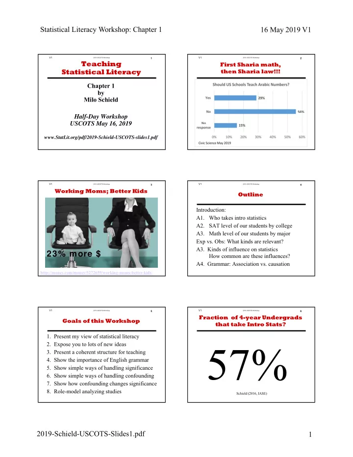
2019 USCOTS Workshop

V1 1

Chapter 1 by Milo Schield Half-Day Workshop USCOTS May 16, 2019

www.StatLit.org/pdf/2019-Schield-USCOTS-slides1.pdf

Teaching Statistical Literacy

2019 USCOTS Workshop

V1

.

2

First Sharia math, then Sharia law!!!

2019 USCOTS Workshop

V1

.

3

Working Moms; Better Kids

23% more $

http://money.com/money/5272659/working-moms-better-kids/

2019 USCOTS Workshop

V1

Introduction:

• A1. Who takes intro statistics
• A2. SAT level of our students by college
• A3. Math level of our students by major

Exp vs. Obs: What kinds are relevant?

• A3. Kinds of influence on statistics

How common are these influences?

• A4. Grammar: Association vs. causation

4

Outline

2019 USCOTS Workshop

V1

• 1. Present my view of statistical literacy
• 2. Expose you to lots of new ideas
• 3. Present a coherent structure for teaching
• 4. Show the importance of English grammar
• 5. Show simple ways of handling significance
• 6. Show simple ways of handling confounding
• 7. Show how confounding changes significance
• 8. Role-model analyzing studies

5

Goals of this Workshop

2019 USCOTS Workshop

V1

Schield (2016, IASE)

6

Fraction of 4-year Undergrads that take Intro Stats?

2019 USCOTS Workshop

V1

Tintle et al, 2013

7

Fraction of Course Gain that Stat Students Loose in 4 Months

2019 USCOTS Workshop

V1

Of those taking Stat I:

• less than 1% take Stat II (10-yrs @ U. St. Thomas)
• less than 0.2% major in statistics (nationwide).
• most see less value in statistics after the course than

they did before. Schield and Schield (2008).

• too many say “Worst course I ever took” [anecdotal]

www.amstat.org/misc/StatsBachelors2003-2013.pdf 1,135 stat majors in 2013 at 32 colleges www.StatLit.org/pdf/2015-Schield-UST-Enroll-in-Statistics.pdf

8

Student Attitudes Toward Stats

2019 USCOTS Workshop

V1

Estimates by Schield (2015, Statchat)

9

What fraction of 4-Yr Intro Stat students are taught outside Math?

2019 USCOTS Workshop

V1

Schield (2016, IASE). Inferred from data in 2012 US Statistical Abstract.

10

Who takes Intro Statistics at Four-Year Colleges?

2019 USCOTS Workshop

V1

Schield (2016, IASE)

11

Where are your students?

2019 USCOTS Workshop

V1

SAT Math Scores: Average by Student Major Percentiles

• f all those

taking the Math SAT

Schield (2016, IASE)

12

SAT Math Percentile by Major

2019 USCOTS Workshop

V1

The real world is complex and can't be described well by one or two variables. If students do not have exposure to simple tools for disentangling complex relationships, they may dismiss statistics as an old-school discipline only suitable for small sample inference of randomized studies.

13

GAISE 2016 Update

2019 USCOTS Workshop

V1

Multivariable thinking is critical to make sense of the observational data around us

• learn to identify observational studies
• learn to consider potential confounding factors
• use … stratification … to show confounding

This report recommends that students be introduced to multivariable thinking, preferably early in the introductory course and not as an afterthought at the end of the course.

14

GAISE 2016 Update

2019 USCOTS Workshop

V1

.

Schield (2016, ASA)

15

Most Important Topics: Student Choices

2019 USCOTS Workshop

V1

Statistical association is not the same as Basketball Assoc. Association words assert association explicitly or describe associations involving fixed conditions or unrepeatable events. Association: Height is associated with age in children Obesity is correlated with (related to) diabetes. Prediction: Graduating from high school predicts success in life.

• *Comparisons: People with degrees earn more than those without

Whites have a higher risk of suicide than blacks. *Co-variation: As children get older, their weight increases.

* Manipulation is impossible, or treatment or outcome cannot be repeated. Schield (2018, SL4DM)

16

A-B-C Words: A = Association

2019 USCOTS Workshop

V1

Causation words assert causation, sufficiency

• r contra-factual

Causation: A bomb caused the fire. Insomnia is a side effect. Lightning resulted in a fire. Spark results in a fire. Sufficient: The more X you do, the more Y you will get. Prevent, stop, end, start, kill, produce, cure, avoid, ban, quit, block, ward off, stave off, cancel, hinder, or eliminate.6 Contra-factual: Those who do X will get more Y than if they had not done X.

17

A-B-C Words: C = Causation

2019 USCOTS Workshop

V1

Between words describe association but imply causation

Verbs: Red wine cuts cancer risk. TV ups kids’ risk of flunking. Gene X increases health risk. Smoking raises asthma risk. Connectors: Nuts linked to cancer. Trauma tied to heart disease. Contributor Diet contributes to diabetes. Age is factor in infertility Nouns: Spinach is asthma protector. Bad water is a killer. Logicals: Anxiety increases due to (because of) high stake testing

• *Compare: People who take antidepressants have fewer migraines

Asthma attacks more likely for smokers than non-smokers. *Covariation: As teacher pay increases, student scores increase. The more hours worked, the more likely a promotion

*Manipulation is possible, and treatment and outcome are repeatable.

18

A-B-C Words: B = Between

2019 USCOTS Workshop

V1

Of the 2,000 news headlines analyzed6, 71% involved A, B or C. Of those headlines involving A, B or C,

• 86% were "between" claims,
• 11% sufficiency, 3% causation, 3% association.
• 6. Schield and Raymond (2009).

19

A-B-C Words: Distribution in Headlines

2019 USCOTS Workshop

V1

This statement is ambiguous. It can mean: 1 Association is not sufficient to prove causation 2 Association provides no evidence for causation. Teachers may intend #1; students often hear #2. A better statement would be: Association is evidence of causation somewhere.

20

Association is not causation

2019 USCOTS Workshop

V1

No idea has stifled the growth of statistical literacy as much as the endless repetition of the words "correlation is not causation". This phrase seems to be primarily used to suppress intellectual inquiry -- by encouraging the unspoken assumption that correlational knowledge is somehow an inferior form of knowledge.

John Myles White (2010):

www.johnmyleswhite.com/notebook/2010/10/01/three-quarter-truths-correlation-is-not-causation/ 21

Association is not causation

2019 USCOTS Workshop

V1 ./ 22

Studies are the Primary Unit of Analysis

2019 USCOTS Workshop

V1 ./ 23

Harvard Case Studies: Title or Abstract

2019 USCOTS Workshop

V1 ./ 24

Statistical Literacy : An Overview

2019 USCOTS Workshop

V1 ./ 25

Stat Literacy studies Stats as Evidence in Arguments

2019 USCOTS Workshop

V1

• Q1. Which group is largest?

Consolidate White (Non-Hispanic) with Hispanic.

• Q2. Which group is largest?

26

Statistical Literacy : Assembly

2019 USCOTS Workshop

V1

Five non-quantitative Topics:

• 1. Regression to the Mean

Sport Illustrated Cover

• 2. Statistically significant
• 3. Chance-Related Mistakes:

Three Door problem; Birthday problem

• Better than chance
• Unlikely to be chance

27

Statistical Literacy : Randomness

2019 USCOTS Workshop

V1

Three kinds of error

• 1. Subject/respondent error:
• 2. Researcher/measurement error:
• 3. Sampling error:

28

Statistical Literacy : Error/Bias

2019 USCOTS Workshop

V1 29

Statistical Literacy : Assembly

2019 USCOTS Workshop

V1

More college students (over half) take intro statistics than any other course (except English). One-size fits all is no longer viable. Statistics education must support Stat 101 and 100/102. Statistics education should (1) support different flavors for different majors, and (2) agree on the contributions of statistics to human knowledge.

/ 30

Statistical Literacy : Recommendation

2019 USCOTS Workshop

V1

The past success of statistics has depended on vast, deliberate simplifications amounting to willful ignorance. This very success now threatens future advances in medicine, the social sciences, and other fields. Limitations of existing methods result in frequent reversals of scientific findings/recommendations, to the consternation of scientists and the public. Herbert I. Weisberg

31

Willful Ignorance

2019 USCOTS Workshop

V1

The past success of statistics has depended on vast, deliberate simplifications amounting to willful ignorance.

32

Willful Ignorance Herbert Weisberg Limitations of existing methods result in frequent reversals of scientific findings and recommendations, to the consternation of scientists and the lay public.

2019 USCOTS Workshop

V1 1

Statistical Literacy Details Chapter 2 by Milo Schield USCOTS Workshop May 16, 2019

www.StatLit.org/pdf/2019-Schield-USCOTS-Slides2.pdf

Statistics Literacy For Decision Makers

2019 USCOTS Workshop

V1

Associations: Comparison and Co-Variation

• Comparisons: Ordered and Arithmetic
• Comparisons: Kinds of Arithmetic

Take CARE: Solutions

• Confounder control: effect size, study design
• Assembly:
• Randomness: Test for statistical significance
• Error/Bias: Single & Double blind.

2

Take CARE: Details Chapter 2 Outline

2019 USCOTS Workshop

V1 ./ 3

Stat Literacy studies Stats as Evidence in Arguments

2019 USCOTS Workshop

V1

Two-group comparisons:

• Men are taller than women
• Women live longer than men

Two-factor Covariation

• As height increases, weight increases
• The more height, the more weight

4

Associations: Two Kinds

2019 USCOTS Workshop

V1

Ordinal (Order): Women live longer than men Arithmetic:

• Men shave six days more/week than women

6% is one percentage point more than the 5%

• Men shave seven times as much as women.
• Men save 600% more often than women.

6% is 20% more than 5%. Men shave six times more often than women. Women shave 7 times less often than men

5

Comparisons: Two Kinds

2019 USCOTS Workshop

V1 ./ 6

Prevalence of Comparisons Google Ngrams

2019 USCOTS Workshop

V1

What things block or negate confounders?

• 1. Large effect size; large arithmetic comparison
• 2. Study design
• 3. Ratios
• 4. Comparison of ratios.
• 5. Selection and stratification
• 6. Standardizing

7

Confounding

2019 USCOTS Workshop

V1

• 1. Does the association involve an effect size?

If not, then no reason to think it is large

• 2. Is the effect size material? For example,

a factor of 10 increase in 1 chance in 10,000.

• 3. Is the effect size statistically significant?
• 4. Is the effect size large enough to ward off

confounders? A: RR>4, B: RR > 3, C: RR>2, D: RR > 1.5. Schield (2018, ICOTS).

8

#1 Effect Size

2019 USCOTS Workshop

V1 ./ 9

Studies are the Primary Unit of Analysis

2019 USCOTS Workshop

V1

There are distinctions within these, but these six are enough to get started.

10

Six Basic Study Designs

2019 USCOTS Workshop

V1

.

11

Study Design Prevalences: Google Ngrams

2019 USCOTS Workshop

V1

Randomized controlled trials (RCT) are a major contribution of statistics to human knowledge. By doing the impossible—controlling for all variations (known and unknown) — randomized trials can be considered a “statistical miracle.” Experiments RCT Gold std. Silver std.

12

Random Assignment Nullifies Prior Confounding

Predictor Result Confounder Association

2019 USCOTS Workshop

V1

• 1747. Lind tests sailors with scurvy.
• 1935 Fisher: The Lady Tasting Tea.
• 1961 Perry Pre-School Project.
• 1974 RAND Health Insurance Experiment
• 1980s First AIDs trial video

13

Random Assignment Examples

2019 USCOTS Workshop

V1

Placebo Effect: Clinical trials where placebo group did as well as treatment group. See migraine prophylaxis, positive response: Placebo meds, 22%. placebo acupuncture 38%. placebo surgery, 58%. Note; Clinical studies, clinically proven, medical trials, medically proven, medical studies and controlled trials don't require randomization.

14

Placebo Effect

2019 USCOTS Workshop

V1 15

Study Designs

562 BC. Jews in Babylon test meat vs vegetarian diet. 1796 Jenner administers cowpox to patient with smallpox 1898 Lease of Hong Kong to the British for 99 years. 1919-1933: US prohibits production/consumption of alcohol.

2019 USCOTS Workshop

V1

1920 Watson's "Little Albert" study of social conditioning. 1945 Post-WWII division of Germany into East and West. 1945/48 Korea partition: North (USSR) and South (USA). 1951 Asch Conformity Exp. 74% agreed w peers' falsehood. 1954 Salk polio vaccine*. Biggest public health experiment. 1968 Bystander Effect. Less likely to act if in a group. 1987-2014: US states allow concealed carry of weapons (CCW)

* Salk: Second graders were treatment group; 1st and 3rd graders were control. www.medicine.mcgill.ca/epidemiology/hanley/c622/salk_trial.pdf

16

Quasi-Experiments: More Examples

2019 USCOTS Workshop

V1

Retrospective longitudinal studies : subjects recall past events. Cheap, quick. Prospective longitudinal studies: follow subjects through time. Expensive, time-consuming. Minimizes recall bias and sampling bias. Cross-sectional results are more reliable. Prospective studies:

• 1921 Terman (Stanford) study of the gifted
• 1948 Framingham Study: Follow all inhabitants of Framingham MA
• 1951 British Doctors Survey
• 1976 Harvard Nurses Study
• 1979 Brouchard study of twins raised apart
• 1979 National Longitudinal Study of Youth (NLSY)

17

Longitudinal Studies: Examples

2019 USCOTS Workshop

V1

• 1948 Framingham Study: Cross-sectional data associated heart

attacks with high blood pressure, high cholesterol and smoking.

• 1951 British Doctors Survey. Cross-sectional data strongly

associated lung-cancer deaths with smoking.

• 1979 Brouchard study of twins raised apart. Similarities

between twins are due more to genes, less to environment.

• 1979 National Longitudinal Study of Youth. Cross-sectional

data showed that social outcomes more strongly associated with individual IQ than with parents’ socio-economic status. See The Bell Curve (1994) by Herrnstein and Murray.

18

Cross Sectional Associations: Examples

2019 USCOTS Workshop

V1

Which are cheapest? Which are most common in the media? Examples of uncontrolled quasi-experiments?

19

Evaluating Study Designs Grades are Starting Points

2019 USCOTS Workshop

V1

Association is not causation vs Association is often evidence of causation. Don’t cross in the middle of the block vs. look both ways before you do. Sex is not love (Danny Kaplan) vs. sex and love can be closely related.

20

From Association to Causation

2019 USCOTS Workshop

V1

The unlikely is almost certain given enough tries Math: Suppose there is one chance in N for a given rare event on the next try. The chance of having at least* one such event in N tries is over 50%—it is expected. * Chance of having just one event < 50%.

21

Chance: Law of Very Large Numbers

2019 USCOTS Workshop

V1

Consider matched statistics from two groups. If their 95% intervals don’t overlap, then their difference is statistically significant. Otherwise, the difference may be statistically insignificant.

22

Chance: Statistical Significance

Suppose 70% of gals dream in color (40% of guys) and the 95% margin of error is 10 points. The associated 95% confidence intervals are 60 to 80% for gals (30 to 50% for guys). The 30 point difference is statistically significant.

2019 USCOTS Workshop

V1

Before 1936, as many as one in three expectant moms died from puerperal fever following birth. Gerhard Domagk, a German doctor, developed Prontosil to fight against streptococcal infections. In 1936, Prontosil was administered to 38 newly delivered mothers, all suffering from puerperal

• fever. Three died and thirty-five survived.

23

Case Study: The Prontosil Experiment

2019 USCOTS Workshop

V1

When Prontosil was administered earlier in the course of the infection, no mother died. In 1936, Prontosil was used to treat Franklin D. Roosevelt, Jr., the President’s son. This was the moment when the world realized that drugs were potent alternatives to surgery.

24

Case Study: The Prontosil Experiment

2019 USCOTS Workshop

V1

Fifty subjects having pain associated with post-polio syndrome were randomly assigned. The treatment group received concentric magnets; the control group received inert placebo magnets. A major decrease in pain was reported by 75% in the treatment group 19% in the control group.

• Natural Health, August, 1998. Page 52.

Effect size. Study design. Hypothetical thinking using Take CARE.

/ 25

Case Study Do Magnets Reduce Pain?

2019 USCOTS Workshop

V1

.

26

Bias or Ignorance?

2019 USCOTS Workshop

V1

.

27

Bias or Ignorance?

2019 USCOTS Workshop

Ch3: V1 1

Chapter 3: Measurements by Milo Schield Half-Day Workshop USCOTS May 16, 2019

www.StatLit.org/pdf/2019-Schield-USCOTS-Slides3.pdf

Statistics Literacy For Decision Makers

2019 USCOTS Workshop

Ch3: V1

Distributions Measures of center Two-group comparisons of Means & Medians Two-variable co-variation Spread Slope and simple regression

2

Measurements: Chapter 3 Outline

2019 USCOTS Workshop

Ch3: V1 ./ 3

Stat Literacy: Study Statistics as Evidence in Arguments

2019 USCOTS Workshop

Ch3: V1

In an asymmetric distribution, mean, median and mode typically align alphabetically with mean most sensitive to extremes. Why?

4

Measures

• f Center

Figure 3D6

Mean Mode Median 50% 50%

100k 200k 300k 400k

Figure 3D7

Hypothetical Distribution

• f Houses by Price

Mean Mode Median

2019 USCOTS Workshop

Ch3: V1

Suppose that house prices in your town have a positive near-symmetric distribution Suppose Bill and Melinda Gates move to your

• town. They built two Mac-Mansions.

How does that change the mode, median and mean of the original distribution? Mode? Median? Mean? Most relevant in the short run? In the long-run?

5

Mean, median, mode:

• Alphabetically. Why?

2019 USCOTS Workshop

Ch3: V1

• 1. Mean is more sensitive to outliers.

Yet statisticians prefer the mean. Why?

• 2. Omit measure: City1 income more than City2.
• 3. Omit characteristic: Midtown is a median city.
• 4. Assume the mean exists. 1.8 kids per family.
• 5. Ambiguity in specifying the group

6

Issues:

2019 USCOTS Workshop

Ch3: V1

.

7

Controlling Confounding: Control Of

2019 USCOTS Workshop

Ch3: V1

.

8

Controlling Confounding: Control For

2019 USCOTS Workshop

Ch3: V1

.

9

Control Of/For Ngrams

2019 USCOTS Workshop

Ch3: V1

A crude association is an association in which nothing else has been taken into account. Less likely to get pregnant:

• Short young adults than tall.
• Adults that shave daily than those that don’t
• Adults with long hair than those with short.

What one takes into account is an assumption. Teachers should say, “Check your assumptions.”

10

Crude Associations

2019 USCOTS Workshop

Ch3: V1

.zxc

11

Crude Association versus an Adjusted Association

US Income Distribution by Quintile Left Bar is Before Adjustment; Right Bar is After

4% 9% 23% 49% 12% 15% 15% 17% 20% 37% 0% 10% 20% 30% 40% 50% Bottom Second Middle Fourth Top Quintile of Families Share (%

• f Total

www.Heritage.org

2019 USCOTS Workshop

Ch3: V1 12

Prison Expense: Crude vs Adjusted Associations

2019 USCOTS Workshop

Ch3: V1

Ratio associations can be still be confounded. Averages are ratios.

13

Crude Ratio Associations It’s the Mix!!!

2019 USCOTS Workshop

Ch3: V1

SAT Verbal flat, but every group improved.

/ 14

Simpson’s Paradox: Time It’s the Mix!!

2019 USCOTS Workshop

Ch3: V1

After learning about Simpson’s Paradox, one student said, "I'll never trust another statistic." This is cynicism: not a good outcome.

15

Will an Association Reverse? The Cornfield Conditions Not all confounders can reverse an association. Jerome Cornfield proved that a confounder association must be "bigger" than the observed. Cornfield's conditions are one of the three biggest contributions of statistics to human knowledge.

2019 USCOTS Workshop

Ch3: V1

.

16

.

SEASON WINS vs. TOTAL PAYROLL

US Major League Baseball 52 62 72 82 92 102 10 20 30 40 50 60 Total Payroll ($Millions) 1995 Season W ins Yankees BlueJays Indians Twins Marlins Rangers Mets Padres Brav es Orioles Red Sox Reds Expos Pirates Tigers

2019 USCOTS Workshop

Ch3: V1

.

17

Regression Standardizes

House Prices (Average Acres = 1.6)

$50,000 $150,000 $250,000 $350,000 $450,000 1 2 3 4 5 6 Land Size (Acres)

2004AssessMTB

Best-Fit Line

2019 USCOTS Workshop

Ch3: V1

The data shows that house prices increase by $39,000 per bedroom. This is a crude association.

18

Regression Standardizes An Example: $16,000 per bedroom if land is controlled for, $9,000 per bedroom after accounting for land and house size, $5,000 after adjusting for land, house size, and number of bathrooms.

2019 USCOTS Workshop

Ch3: V1

Children under two should not be allowed to watch television because it increases their chances

• f suffering attention problems later in life, says

an American study. A study of 1,345 children found that each hour spent in front of the set every day increased the risks of attention deficit disorders by 10%.

U.S. journal, Pediatrics

19

TV for toddlers interferes with brain growth, says study:

2019 USCOTS Workshop

Ch3: V1

If a child’s risk of Attention Deficit Disorder increases by 10% for every extra hour of watching TV, how many hours do they have to watch to double their risk?

20

Time to Double given Growth Rate Rule of 72*: Time to double = 72 / Rate 72 divided by 10% per hour = 7.2 hours * Assuming compounding

2019 USCOTS Workshop

Ch3: V1

Don’t talk about confounding or effect size. Talk about assumptions.

• What one controls for is an assumption.
• What one fails to control for is an assumption.

AAU&C Quantitative Literacy VALUE rubric: Assumptions: Ability to make and evaluate important assumptions in estimation, modeling, and data analysis.

21

How to Relate this to Math Colleagues

2019 USCOTS Workshop

Ch3: V1

Interpretation, Representation, Calculation, Application, Assumptions, and Communication Assumptions: Ability to make and evaluate important assumptions in estimation, modeling, and data analysis.

www.statlit.org/pdf/2009QuantitativeLiteracyRubricAACU.pdf www.aacu.org/peerreivew/2014/summer/RealityCheck

22

AAC&U Quantitative Literacy VALUE Rubric

2019 USCOTS Workshop

Ch4: V1 1

Chapter 4: Using and Describing Ratios by Milo Schield Half-Day Workshop USCOTS May 16, 2019

www.StatLit.org/pdf/2019-Schield-USCOTS-Slides4.pdf

Teaching Statistical Literacy

2019 USCOTS Workshop

Ch4: V1

.

2

Workshop Schedule

2019 USCOTS Workshop

Ch4: V1

Per grammars:

• Percent grammar
• Percentage grammar
• Reading half tables and tables w/o margins
• Rate grammar

Ordinary Preposition grammars:

• Chance grammar
• Ratio grammar

3

Ratios: Chapter 4 Outline

2019 USCOTS Workshop

Ch4: V1 ./ 4

Stat Literacy: Study Statistics as Evidence in Arguments

2019 USCOTS Workshop

Ch4: V1

• 1. One in five children face hunger [2019 billboard in St. Paul]
• 2. Two absences per month = Likely to fail a grade
• 3. Ninth-grade attendance better predicts graduation than 8th

grade test score

• 4. Attendance alone explains 31% of the variance in performance
• 5. Budget cuts lead to deaths in Federal prisons
• 6. 22 million victims of human trafficking trapped worldwide.
• 7. The National Rifle Association is a terrorist organization.
• 8. Ban assault weapons
• 9. 2016 Memphis. 228 homicides. Down 500 police officers.

5

Evaluate these Using Just Assembly/Assumptions

2019 USCOTS Workshop

Ch4: V1

.

6

Forming Ratios

2019 USCOTS Workshop

Ch4: V1

.

7

From Comparisons to Ratios: Using Prepositions

2019 USCOTS Workshop

Ch4: V1

.

8

.

2019 USCOTS Workshop

Ch4: V1

.

9

Prevalence of Named Ratios

2019 USCOTS Workshop

Ch4: V1

Which kind of percents are these: part-whole or percent compare?

• 1. The youngest child's share of the candy.
• 2. Interest charged per year by the Mafia (criminals).
• 3. People live 100% longer on average in US than in Swaziland.
• 4. The advertisement said "40% off".

.

10

Two Kinds of Percents

2019 USCOTS Workshop

Ch4: V1

Of all adults. .

11

Part-Whole Using Pie Charts

2019 USCOTS Workshop

Ch4: V1

• 1. 40% of US adults did not vote for president in 2016.
• 2. The percentage of US adults who didn’t vote was 40%
• 3. The non-voter rate among US adults in 2016 was 40%.
• 4. There was a 40% chance that an adult was a non-voter.

.

12

Four Different Grammars; Confusion of the Inverse

• Confusion of the inverse exchanges part with whole.
• 1. “The percentage of men who are in the military”

.NE. “the percentage of the military who are men”.

• 2. The percentage of smokers among women .NE.

“the percentage of smokers who are women”.

2019 USCOTS Workshop

Ch4: V1

Describe the 30% Describe the 36%

13

Use Percent Grammar <X% of Whole are Part>

2019 USCOTS Workshop

Ch4: V1

• 1. What percentage of men are art majors?
• 2. What percentage of art majors are men?
• 3. What percentage of students are male art majors?

14

Tables: Use Percent Grammar <X% of Whole are Part>

2019 USCOTS Workshop

Ch4: V1

Describe the 10% Describe the 5%

15

100% Tables: Percent Grammar <X% of Whole are Part>

2019 USCOTS Workshop

Ch4: V1

.

16

Use Percent Grammar <X% of Whole are Part>

2019 USCOTS Workshop

Ch4: V1

• 1. The percentage of seniors who smoke is 15%.
• 2. Among seniors, the percentage who smoke is 15%.
• 3. Among Seniors, the percentage of smokers is 20%.
• 4. Among men, the percentage of seniors who smoke is 20%

Numbers 3 and 4 are problems. “Of” introduces whole in percent grammar.

17

Percentage Grammar Four form

2019 USCOTS Workshop

Ch4: V1

Sports grammar is readily understood with a natural whole:

• percentage of defective cans; percentage of tire failures

Without a natural whole, sports grammar is ambiguous.

• percentage of female smokers;
• percentage of working males
• percentage of infant deaths;
• percentage of single mothers

18

Percentage Grammar Sports Grammar

2019 USCOTS Workshop

Ch4: V1

Describe the circled 60%. Use percent grammar.

19

Half Tables when Parts of 100% Table are Binary If 60% returned, what percentage did not return? So, the right two columns are redundant. Eliminating them will save space!

2019 USCOTS Workshop

Ch4: V1

.

20

Confounding

2019 USCOTS Workshop

Ch 13: V1 1

13: Confounding & Cornfield by Milo Schield Half-Day Workshop USCOTS May 16, 2019

www.StatLit.org/pdf/2019-Schield-USCOTS-Slides13.pdf

Statistics Literacy For Decision Makers

2019 USCOTS Workshop

Ch 13: V1

1:00 Ch 1 Statistical Literacy – Introduction 1:30 Ch 2 Statistical Literacy – Details 2:15 Ch 3 Measurements 2:45 Ch 4 Ratios 3:30 Ch 13 Standardizing 4:00 Feedback .

2

Workshop Schedule

2019 USCOTS Workshop

Ch 13: V1

Cornfield-Fisher debate Cornfield conditions Standardizing percentages, rates and averages Standardizing percentage & number attributable Statistical significance and confounding

3

Confounding: Chapter 13 Outline

2019 USCOTS Workshop

Ch 13: V1 ./ 4

Stat Literacy: Study Statistics as Evidence in Arguments

2019 USCOTS Workshop

Ch 13: V1

Doctors had noticed the strong association between smoking and lung cancer. Statisticians argued that this evidence strongly supported the claim that smoking was a cause of lung cancer. Fisher, a smoker, noted that association is not causation in observational studies. Fisher produced data. Identical twins were more likely to share a smoking preference than were fraternal twins. This statistic supported genetics as an alternate explanation for the association.

5

Cornfield-Fisher Debate

2019 USCOTS Workshop

Ch 13: V1

Now when the world’s leading statistician says something that every statistician agrees is true, most reasonably-minded statisticians would back off. And when the world’s leading statistician produces data indicating a plausible confounder, it seems incredible that anyone would reply. Jerome Cornfield did!

6

Cornfield-Fisher Debate

2019 USCOTS Workshop

Ch 13: V1

Cornfield proved that the relative risk of lung cancer had to be greater for a confounder (e.g., genetics) than for the predictor (e.g., smoking) in order to nullify or reverse the observed association. Cornfield pointed out that smokers were about 10 times as likely to get lung cancer as non-smokers. Fisher’s data involved a factor of two. Fisher never replied.

7

Cornfield Conditions

2019 USCOTS Workshop

Ch 13: V1

“Cornfield's minimum effect size is as important to

• bservational studies as is the use of randomized

assignment to experimental studies. No longer could one refute an ostensive causal association by simply asserting that some new factor (such as a genetic factor) might be the true cause. Now one had to argue that the relative prevalence of this potentially confounding factor was greater than the relative risk for the ostensive cause.”

Schield (1999). [This was written 20 years ago!]

8

Contributions to Human Knowledge

2019 USCOTS Workshop

Ch 13: V1

Since confounders may be unknown, there is no way to derive or infer their distribution. Schield (2018) argued that we needed a standard for confounder: a standard confounder distribution. He proposed an exponential (one factor determined)

with a mean relative risk of 2. This applied if predictor and confounder are binary.

9

Confounder Distribution

2019 USCOTS Workshop

Ch 13: V1 10

Confounder Distribution Unknown & Unknowable

2019 USCOTS Workshop

Ch 13: V1

Wainer introduced a simple graphical technique that made the control of a binary confounder a relatively simple matter. Schield (2006). Presenting Confounding Graphically Using Standardization, STATS magazine. www.statlit.org/pdf/2006SchieldSTATS.pdf

11

Controlling for a Confounder: Graphical Technique

2019 USCOTS Workshop

Ch 13: V1

.

12

Crude Association: Death Rate: City > Rural

A Confounder can Influence a Difference

0% 1% 2% 3% 4% 5% 6% 7% 0% 20% 40% 60% 80% 100%

Percentage who are in "Poor" Condition

Death Rate

2019 USCOTS Workshop

Ch 13: V1

.

13

Controlling for a Confounder: Death Rate: City < Rural

Standardizing Can Reverse A Difference

0% 1% 2% 3% 4% 5% 6% 7% 0% 20% 40% 60% 80% 100%

Percentage who are in "Poor" Condition

Death Rate

2019 USCOTS Workshop

Ch 13: V1

.

14

Crude Association: Statistically Significant

Percentage of Babies who have low Birth-Weight

5% 7% 9% 11% 13% 15% 17% 0% 10% 20% 30% 40% 50% 60% 70% 80% 90% 100%

Percentage of Moms who are Under 19

Low Birth Weights

Mom didn't smoke

Mom smoked

2019 USCOTS Workshop

Ch 13: V1

.

15

Standardized Association: Statistically Insignificant

Percentage of Babies who have low Birth-Weight

5% 7% 9% 11% 13% 15% 17% 0% 10% 20% 30% 40% 50% 60% 70% 80% 90% 100%

Percentage of Moms who are Under 19

Low Birth Weights

Mom didn't smoke

Mom smoked Standardized

2019 USCOTS Workshop

Ch 13: V1

Controlling for a confounder can transform a statistically-significant association into an association that is statistically insignificant.

Although statistical educators are clearly aware of this, there is nothing in any introductory textbook that alerts students to this possibility. The failure to show a significance reversal is statistical negligence.

16

Confounder Effect on Statistical Significance