533d animation physics why
play

533D Animation Physics: Why? Natural phenomena: passive motion - PowerPoint PPT Presentation

533D Animation Physics: Why? Natural phenomena: passive motion Film/TV: difficult with traditional techniques CS533D - Animation Physics When you control every detail of the motion, it s hard to make it look like it s not being


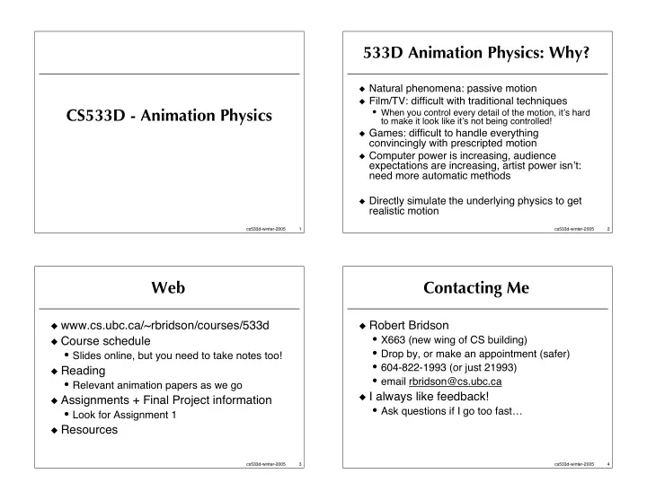
  1. 533D Animation Physics: Why? � Natural phenomena: passive motion � Film/TV: difficult with traditional techniques CS533D - Animation Physics • When you control every detail of the motion, it � s hard to make it look like it � s not being controlled! � Games: difficult to handle everything convincingly with prescripted motion � Computer power is increasing, audience expectations are increasing, artist power isn � t: need more automatic methods � Directly simulate the underlying physics to get realistic motion cs533d-winter-2005 1 cs533d-winter-2005 2 Web Contacting Me � www.cs.ubc.ca/~rbridson/courses/533d � Robert Bridson • X663 (new wing of CS building) � Course schedule • Drop by, or make an appointment (safer) • Slides online, but you need to take notes too! • 604-822-1993 (or just 21993) � Reading • email rbridson@cs.ubc.ca • Relevant animation papers as we go � I always like feedback! � Assignments + Final Project information • Ask questions if I go too fast… • Look for Assignment 1 � Resources cs533d-winter-2005 3 cs533d-winter-2005 4

  2. Evaluation Topics � 4 assignments (60%) � Particle Systems • See the web for details + when they are due • the basics - time integration, forces, collisions • Mostly programming, with a little analysis (writing) � Deformable Bodies � Also a final project (40%) • e.g. cloth and flesh • Details will come later, but basically you need to � Constrained Dynamics either significantly extend an assignment or animate something else - talk to me about topics • e.g. rigid bodies • Present in final class - informal talk, show movies � Fluids � Late: without a good reason, 20% off per day • e.g. water • For final project starts after final class • For assignments starts morning after due cs533d-winter-2005 5 cs533d-winter-2005 6 Particle Systems Particle Systems � Read: Reeves, “Particle systems…”, SIGGRAPH � 83 Sims, “Particle animation and rendering using data parallel computation", SIGGRAPH '90 Miller & Pearce, “Globular dynamics…”, SIGGRAPH � 89 � Some phenomena is most naturally described as many small particles • Rain, snow, dust, sparks, gravel, … � Others are difficult to get a handle on • Fire, water, grass, … cs533d-winter-2005 7 cs533d-winter-2005 8

  3. Particle Basics Example � Each particle has a position � Sparks from a campfire • Maybe orientation, age, colour, velocity, � Every frame (1/24 s) add 2-3 particles temperature, radius, … • Position randomly in fire • Call the state x • Initialize temperature randomly � Seeded randomly somewhere at start � Move in specified turbulent smoke flow • Maybe some created each frame • Also decrease temperature � Move (evolve state x) each frame � Render as a glowing dot (blackbody according to some formula radiation from temperature) � Eventually die when some condition met � Kill when too cold to glow visibly cs533d-winter-2005 9 cs533d-winter-2005 10 Rendering First Order Motion � We won � t talk much about rendering in this course, but most important for particles � The real strength of the idea of particle systems: how to render • Could just be coloured dots • Or could be shards of glass, or animated sprites (e.g. fire), or deforming blobs of water, or blades of grass, or birds in flight, or … cs533d-winter-2005 11 cs533d-winter-2005 12

  4. First Order Motion Forward Euler � For each particle, have a simple 1 st order � Simplest method: x n + 1 � x n differential equation: ( ) = v x n , t n � t dx ( ) dt = v x , t Or: ( ) x n + 1 = x n + � tv x n , t n � Analytic solutions hopeless � Need to solve this numerically forward in � Can show it � s first order accurate: time from x(t=0) to • Error accumulated by a fixed time is O( � t) x(frame1), x(frame2), x(frame3), … � Thus it converges to the right answer • May be convenient to solve at some • Do we care? intermediate times between frames too cs533d-winter-2005 13 cs533d-winter-2005 14 Aside on Error Forward Euler Stability � General idea - want error to be small � Big problem with Forward Euler: • Obvious approach: make � t small it � s not very stable dx dt = � x , x (0) = 1 • But then need more time steps - expensive � Example: � Also note - O(1) error made in modeling e � t � Real solution smoothly decays to zero, • Even if numerical error was 0, still wrong! always positive • In science, need to validate against experiments • In graphics, the experiment is showing it to an � Run Forward Euler with � t=11 audience: does it look real? • x=1, -10, 100, -1000, 10000, … � So numerical error can be huge, as long as your • Instead of 1, 1.7*10 -5 , 2.8*10 -10 , … solution has the right qualitative look cs533d-winter-2005 15 cs533d-winter-2005 16

  5. Linear Analysis The Test Equation � Get a rough, hazy, heuristic picture of the � Approximate stability of a method ) + � v � x � ( x � x � ) + � v ( ( ) � v x � , t � � t � ( t � t � ) v x , t � Note that eigenvalue � can be complex � But, assume that for real physics � Ignore all but the middle term (the one that • Things don � t blow up without bound could cause blow-up) • Thus real part of eigenvalue � is � 0 � Beware! dx dt = Ax • Nonlinear effects can cause instability • Even with linear problems, what follows assumes � Look at x parallel to eigenvector of A: constant time steps - varying (but supposedly stable) dx dt = � x the “test equation” steps can induce instability � see J. P. Wright, “Numerical instability due to varying time steps…”, JCP 1998 cs533d-winter-2005 17 cs533d-winter-2005 18 Using the Test Equation Stability Region � Can plot all the values of � � t on the � Forward Euler on test equation is x n + 1 = x n + � t � x n complex plane where F.E. is stable: � Solving gives n x 0 ( ) x n = 1 + � � t � So for stability, need 1 + � � t < 1 cs533d-winter-2005 19 cs533d-winter-2005 20

  6. Real Eigenvalue Imaginary Eigenvalue � Say eigenvalue is real (and negative) � If eigenvalue is pure imaginary… • Corresponds to a damping motion, smoothly • Oscillatory or rotational motion coming to a halt � Cannot make � t small enough � Then need: � t < 2 � Forward Euler unconditionally unstable for � these kinds of problems! � Is this bad? � Need to look at other methods • If eigenvalue is big, could mean small time steps • But, maybe we really need to capture that time scale anyways, so no big deal cs533d-winter-2005 21 cs533d-winter-2005 22 Runge-Kutta Methods Midpoint RK2 � Second order: error is O( � t 2 ) when smooth � Also “explicit” • next x is an explicit function of previous � Larger stability region: � But evaluate v at a few locations to get a better estimate of next x � E.g. midpoint method (one of RK2) ( ) x n + 12 = x n + 1 2 � tv x n , t n ( ) x n + 1 = x n + � tv x n + 12 , t n + 12 � But still not stable on imaginary axis: no point cs533d-winter-2005 23 cs533d-winter-2005 24

  7. Modified Euler Modified Euler (2) � Stability region for � =2/3 � (Not an official name) � Lose second-order accuracy, get stability on imaginary axis: ( ) x n + � = x n + � � tv x n , t n ( ) x n + 1 = x n + � tv x n + � , t n + � � Parameter � between 0.5 and 1 gives � Great! But twice the cost of Forward Euler trade-off between imaginary axis and real � Can you get more stability per v- axis evaluation? cs533d-winter-2005 25 cs533d-winter-2005 26 Higher Order Runge-Kutta TVD-RK3 � RK3 and up naturally include part of the � RK3 useful because it can be written as a imaginary axis combination of Forward Euler steps and averaging: can guarantee some properties even for nonlinear problems! ( ) n + 1 = x n + � tv x n , t n ˜ x ( ) n + 2 = ˜ n + 1 + � tv ˜ ˜ x x x n + 1 , t n + 1 n + 12 = 3 4 x n + 1 ˜ 4 ˜ x x n + 2 ( ) n + 32 = ˜ n + 12 + � tv ˜ ˜ x x x n + 12 , t n + 12 x n + 1 = 1 3 x n + 2 3 ˜ x n + 32 cs533d-winter-2005 27 cs533d-winter-2005 28

  8. RK4 Selecting Time Steps � Often most bang for the buck ( ) v 1 = v x n , t n ( ) v 2 = v x n + 1 2 � tv 1 , t n + 12 ( ) v 3 = v x n + 1 2 � tv 2 , t n + 12 ( ) v 4 = v x n + � tv 3 , t n + 1 ( ) x n + 1 = x n + � t 6 v 1 + 2 6 v 2 + 2 6 v 3 + 1 1 6 v 4 cs533d-winter-2005 29 cs533d-winter-2005 30 Selecting Time Steps Time Stepping � Hack: try until it looks like it works � Sometimes can pick constant � t • One frame, or 1/8th of a frame, or … � Stability based: • Figure out a bound on magnitude of Jacobian � Often need to allow for variable � t • Changing stability limit due to changing Jacobian • Scale back by a fudge factor (e.g. 0.9, 0.5) • Difficulty in Newton converging � Try until it looks like it works… (remember all the dubious assumptions we made for linear stability • … analysis!) � But prefer to land at the exact frame time � Why is this better than just hacking around in the • So clamp � t so you can � t overshoot the frame first place? � Adaptive error based: • Usually not worth the trouble in graphics cs533d-winter-2005 31 cs533d-winter-2005 32

Download Presentation
Download Policy: The content available on the website is offered to you 'AS IS' for your personal information and use only. It cannot be commercialized, licensed, or distributed on other websites without prior consent from the author. To download a presentation, simply click this link. If you encounter any difficulties during the download process, it's possible that the publisher has removed the file from their server.

Recommend


More recommend