: 5.1.2 - PowerPoint PPT Presentation

הביקע

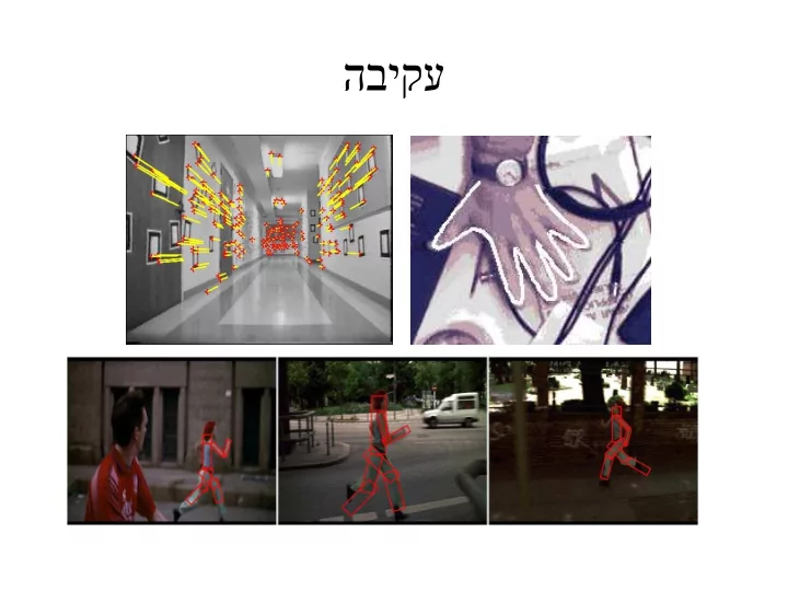
רועישב רמוחל תורוקמ • דומילה רפס : – קרפ 5.1.2 • Forsyth & Ponce קרפ 18 – • םינוש םירמאמ • טנרטניאב רמוח !

Today • …Tracking with Dynamics – Detection vs. Tracking – Tracking as probabilistic inference – Prediction and Correction • Linear Dynamic Models • The Kalman Filter – Kalman filter for 1D state – General Kalman filter – Limitations

Detection vs. Tracking … t=1 t=2 t=20 t=21

Detection vs. Tracking … t=1 t=2 t=20 t=21 • Detection – We detect the object independently in each frame and can record its position over time, e.g., based on blob’s centroid or detection window coordinates.

Detection vs. Tracking … t=1 t=2 t=20 t=21 • Tracking with dynamics : – We use image measurements to estimate the object position, but also incorporate the position predicted by dynamics, i.e., our expectation of the object’s motion pattern.

Tracking with Dynamics • Key idea – Given a model of expected motion, predict where objects will occur in next frame, even before seeing the image. – In next frame, update prediction using actual measurements

Illustration initial position prediction measurement update y y y y x x x x

Tracking with Dynamics • Key idea – Given a model of expected motion, predict where objects will occur in next frame, even before seeing the image. – In next frame, update prediction using actual measurements • Goals – Restrict search for the object – Improved estimates since measurement noise is reduced by trajectory smoothness. • Assumption: continuous motion patterns – Camera is not moving instantly to new viewpoint. – Objects do not disappear and reappear in different places. – Gradual change in pose between camera and scene.

General Model for Tracking state x 1 state x 1 state state x 2 state x 2 state x 3 state x 3 state x 4 state x 4 measurement y 1 y 2 y 3 y 4

General Model for Tracking • The moving object of interest is characterized by an underlying state X • State X gives rise to measurements or observations Y • At each time t , the state changes to X t and we get a new observation Y t … X 1 X 2 X t Y 1 Y 2 Y t

State vs. Observation • Hidden state : parameters of interest (e.g., location of point, contour of shape, etc.) • Measurement : what we get to directly observe (e.g., pixel values, image features)

Tracking as Inference • Our goal: recover most likely state X t given – All observations seen so far. – Knowledge about dynamics of state transitions. • In other words maximize ( | ) p x y t 1... t • Different approaches include: – HMMs – Kalman filters – Condensation

Steps of tracking • Prediction: What is the next state of the object given past measurements?       , , P X Y y Y y  0 0 1 1 t t t

Steps of tracking • Prediction: What is the next state of the object given past measurements?       , , P X Y y Y y  0 0 1 1 t t t • Correction: Compute an updated estimate of the state from prediction and measurements       , , , P X Y y Y y Y y   0 0 1 1 t t t t t

Steps of tracking • Prediction: What is the next state of the object given past measurements?       , , P X Y y Y y  0 0 1 1 t t t • Correction: Compute an updated estimate of the state from prediction and measurements       , , , P X Y y Y y Y y   0 0 1 1 t t t t t

Simplifying assumptions • Only the immediate past matters        , , P X X X P X X  0 1 1 t t t t dynamics model

Simplifying assumptions • Only the immediate past matters        , , P X X X P X X  0 1 1 t t t t dynamics model • Measurements depend only on the current state       , , , , P Y X Y X Y X P Y X   0 0 1 1 t t t t t t observation model

Simplifying assumptions • Only the immediate past matters        , , P X X X P X X  0 1 1 t t t t dynamics model • Measurements depend only on the current state       , , , , P Y X Y X Y X P Y X   0 0 1 1 t t t t t t observation model … X 1 X 2 X t X t-1 Y 1 Y 2 Y t Y t-1

Tracking as Induction • Base case:  Assume we have initial prior that predicts state in absence of any evidence: P ( X 0 ) Perceptual and Sensory Augmented Computing  At the first frame , correct this given the value of Y 0 = y 0 ( | ) ( ) P y X P X    0 0 0 ( | ) ( | ) ( ) P X Y y P y X P X 0 0 0 0 0 0 ( ) P y Computer Vision WS 08/09 0 Posterior prob. Likelihood of Prior of of state given measurement the state measurement

Tracking as Induction • Base case:  Assume we have initial prior that predicts state in absence of any evidence: P ( X 0 ) Perceptual and Sensory Augmented Computing  At the first frame , correct this given the value of Y 0 = y 0 • Given corrected estimate for frame t :  Predict for frame t +1  Correct for frame t +1 Computer Vision WS 08/09 predict correct

Induction Step: Prediction   • Prediction involves representing  , , P X y y    0 1 t t given  , , P X y y   1 0 1 t t Perceptual and Sensory Augmented Computing    , , P X y y  0 1 t t      , , , P X X y y dX    1 0 1 1 t t t t      Computer Vision WS 08/09  Law of total probability   | , , , | , , P X X y y P X y y dX      1 0 1 1 0 1 1 t t t t t t       , P A P A B dB        | | , , P X X P X y y dX     1 1 0 1 1 t t t t t

Induction Step: Prediction   • Prediction involves representing  , , P X y y    0 1 t t given  , , P X y y   1 0 1 t t Perceptual and Sensory Augmented Computing    , , P X y y  0 1 t t      , , , P X X y y dX    1 0 1 1 t t t t      Computer Vision WS 08/09    | , , , | , , P X X y y P X y y dX      1 0 1 1 0 1 1 t t t t t t       Conditioning on X t – 1  | | , , P X X P X y y dX       1     1 0 1 1 t t t t t  , | P A B P A B P B

Induction Step: Prediction   • Prediction involves representing  , , P X y y    0 1 t t given  , , P X y y   1 0 1 t t Perceptual and Sensory Augmented Computing    , , P X y y  0 1 t t      , , , P X X y y dX    1 0 1 1 t t t t      Computer Vision WS 08/09    | , , , | , , P X X y y P X y y dX      1 0 1 1 0 1 1 t t t t t t        | | , , P X X P X y y dX     1 1 0 1 1 t t t t t Independence assumption

Induction Step: Correction   • Correction involves computing 0  , , P X y y   t t given predicted value  , , P X y y  0 1 t t   Perceptual and Sensory Augmented Computing 0  , , P X y y t t       | , , , | , , P y X y y P X y y    0 1 0 1 t t t t t    | , , P y y y  0 1 t t     Computer Vision WS 08/09  | | , , P y X P X y y Bayes rule   0 1 t t t t        | , , P y y y | P B A P A     0 1 t t | P A B       P B  | | , , P y X P X y y   0 1 t t t t       | | , , P y X P X y y dX  0 1 t t t t t

Induction Step: Correction   • Correction involves computing 0  , , P X y y   t t given predicted value  , , P X y y  0 1 t t   Perceptual and Sensory Augmented Computing 0  , , P X y y t t       | , , , | , , P y X y y P X y y    0 1 0 1 t t t t t    | , , P y y y  0 1 t t     Computer Vision WS 08/09  | | , , P y X P X y y   0 1 t t t t    | , , P y y y  0 1 t t      | Independence assumption | , , P y X P X y y   0 1 t t t t (observation y t depends only on state X t )       | | , , P y X P X y y dX  0 1 t t t t t