3.3: Time Series and Index Numbers 1. Time series: Plots - PowerPoint PPT Presentation

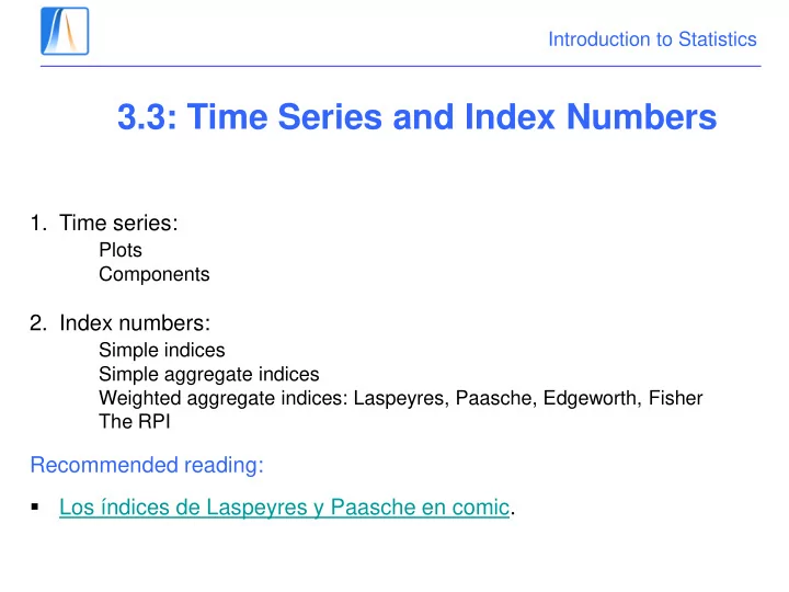
Introduction to Statistics 3.3: Time Series and Index Numbers 1. Time series: Plots Components 2. Index numbers: Simple indices Simple aggregate indices Weighted aggregate indices: Laspeyres, Paasche, Edgeworth, Fisher The RPI Recommended reading:  Los índices de Laspeyres y Paasche en comic.

Introduction to Statistics Motivation Thus far, we have studied the characteristics of a sample of data. However, in many situations, these characteristics can change over time: Unemployment, inflation, the price of beer, consumption of ice-creams We want to study the changes in the value of a variable over time.

Introduction to Statistics Time Series ¿What is a time series? It is a set of measures, ordered according to a time index, of a variable of interest. Número de encarcelados Año 1987 26905 1988 28917 1989 30947 ¿How does the population of prisoners change over 1990 33035 time? 1991 36512 1992 40950 1993 45341 1994 48201 1995 45198 1996 44312 1997 43453 1998 44747 1999 45384 2000 45309 Números de encarcelados por año en España tomados de Eurostat

Introduction to Statistics The time series graph 60000 50000 40000 Número de encarcelados 30000 20000 10000 0 1986 1988 1990 1992 1994 1996 1998 2000 2002 Año ¿What are the characteristics of this series?

Introduction to Statistics Characteristics of time series 250 A monthly series of 200 beer production in Australia. There is a strong seasonal Producción de cerveza 150 effect and a positive trend in the first part of the 100 series. 50 0 1950 1955 1960 1965 1970 1975 1980 1985 1990 1995 2000 Año

Introduction to Statistics Decomposition of time series How do we estimate the trend and seasonal effects? Suppose an additive model y t = T t + E t + I t 250 The trend can be estimated using 200 regression or moving averages. Producción de cerveza 150 100 50 0 1950 1955 1960 1965 1970 1975 1980 1985 1990 1995 2000 Año

Introduction to Statistics Now we take the trend out of the series… 40 30 20 10 yt-Tt 0 1950 1955 1960 1965 1970 1975 1980 1985 1990 1995 2000 -10 -20 -30 -40 Año

Introduction to Statistics and calculate the seasonal effect… 40 30 20 10 0 E 1950 1955 1960 1965 1970 1975 1980 1985 1990 1995 2000 -10 -20 -30 -40 Año

Introduction to Statistics Getting rid of the seasonal effect we are left with a series of irregular variations. 30 20 10 0 1950 1955 1960 1965 1970 1975 1980 1985 1990 1995 2000 I -10 -20 -30 -40 Año

Introduction to Statistics Index Numbers An index number is an indicator designed to describe the changes in a variable over time, that is its evolution over a given time period. • the evolution in the quantity of a determined product or service or of a group of products or services (e.g. quantities produced or consumed). • the changes in the price of a product or service or a group of such. • the changes in the value of a product or service or a basket of such.

Introduction to Statistics Simple indices We want to look at the changes in the prisoner population relative to the year 1987. Número de encarcelados Índice Año 1987 26905 100 1988 28917 107,478164 1989 30947 115,02323 1990 33035 122,783869 The number of prisoners 1991 36512 135,707118 in 2000 has increased 1992 40950 152,202193 by 68% with respect to 1993 45341 168,522579 the prisoner population 1994 48201 179,152574 in1987. 1995 45198 167,99108 1996 44312 164,698012 1997 43453 161,505296 1998 44747 166,314811 1999 45384 168,682401 2000 45309 168,403642 = (45309/26905)*100%

Introduction to Statistics Aggregate indices In many occasions, we are not interested in comparing the prices (quantities or values) of individual goods, but in comparing these for groups of products. Article Prices Simple indices Year 2007 2009 2007 2009 Milk 10 12 100 120 Cheese 15 20 100 133,3 Butter 80 80 100 100

Introduction to Statistics Simple aggregate indices The most basic index is simply the arithmetic mean of all the indices I 2009 = (120+133,3+100)/3 = 117,76 Alternatives are geometric or harmonic means or aggregate indices. What is the problem with this type of index?

Introduction to Statistics They don’t take the consumption of each product into account. Article Prices Units consumed Year 2007 2009 2007 2009 Milk 10 12 50 40 Cheese 15 20 20 10 Butter 80 80 1 1

Introduction to Statistics Weighted aggregate indices I: Laspeyres index We suppose that the consumption in year t is the same as that in the base year. old quantities * new prices old quantities * old prices

Introduction to Statistics Weighted aggregate indices II: Paasche’s index We suppose that consumption in the base year is the same as in year t. new quantities * new prices new quantities * old prices

Introduction to Statistics Weighted indices III: Fisher and Edgeworth Fisher’s index is the geometric mean of Laspeyres and Paasche The Edgeworth index uses the sum of the quantities consumed in the base year and in year t as the weight.

Introduction to Statistics The Retail or Consumer Price index (RPI) Describes the evolution of prices of consumption over time. Every 10 years, a survey (EPF) is taken to analyze the spending habits of a large number of families. The consumption of various products which form the typical shopping basket is considered. In the following years a Laspeyres index based on the consumption in the EPF year is calculated. In the majority of the developed world, the RPI increases over time.

Introduction to Statistics Example The diagram shows a monthly time series of airline passengers for a particular company in the 1950’s. The characteristics of this series are. a) It is stationary. b) It shows a seasonal effect but no trend. c) It shows seasonal and trend effects. d) It shows a trend but no seasonality.

Introduction to Statistics Example The table shows the prices and quantities of burgers and milkshake bought, on average, per day in a Madrid bar in the years 2005 to 2007. Taking the base year as 2005: a) The Laspeyres index for 2005 is 150%. b) The Laspeyres index for 2006 is 150%. c) The Laspeyres index for 2007 is 150%. d) None of the above.