2017-07-29 codon substitution models and the analysis of natural - - PDF document

2017-­‑07-­‑29 ¡ 1 ¡ codon substitution models and the analysis of natural selection pressure

Joseph P. Bielawski Department of Biology Department of Mathematics & Statistics Dalhousie University

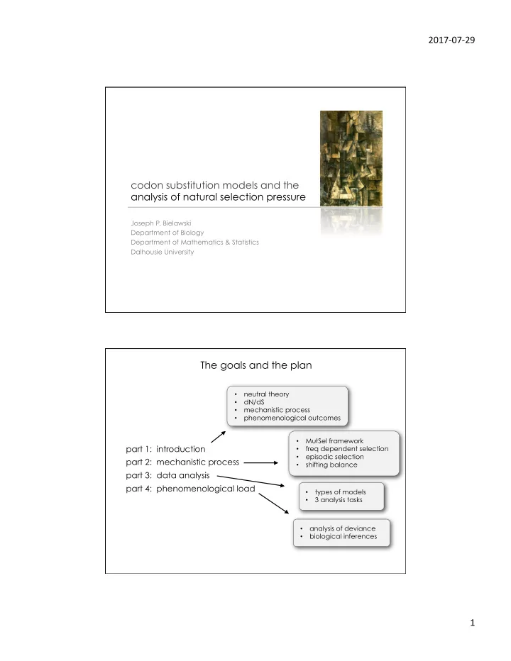
The goals and the plan

v ¡

• types of models
• 3 analysis tasks

v ¡

• MutSel framework
• freq dependent selection
• episodic selection
• shifting balance

v ¡

• neutral theory
• dN/dS
• mechanistic process
• phenomenological outcomes

part 1: introduction part 2: mechanistic process part 3: data analysis part 4: phenomenological load

v ¡

• analysis of deviance
• biological inferences

2017-­‑07-­‑29 ¡ 2 ¡

part 1: introduction

macroevolutioanry time-scale population time-scale

GTG CTG TCT CCT GCC GAC AAG ACC AAC GTC AAG GCC GCC TGG GGC AAG GTT GGC GCG CAC ... ... ... G.C ... ... ... T.. ..T ... ... ... ... ... ... ... ... ... .GC A.. ... ... ... ..C ..T ... ... ... ... A.. ... A.T ... ... .AA ... A.C ... AGC ... ... ..C ... G.A .AT ... ..A ... ... A.. ... AA. TG. ... ..G ... A.. ..T .GC ..T ... ..C ..G GA. ..T ... ... ..T C.. ..G ..A ... AT. ... ..T ... ..G ..A .GC ...

conserved sites: slower than neutral? fast sites: neutral? or faster than neutral?

selectively constrained = slower than neutral (drift alone) adaptive divergence = faster than neutral (drift alone)

What is the neutral expectation?

evolutionary rate depends on intensity of selection

2017-­‑07-­‑29 ¡ 3 ¡

v ¡ v ¡

neutral theory of molecular evolution (Kimura 1968)

the number of new mutations arising in a diploid population v ¡

2Nµ

the fixation probability of a new mutant by drift

12N

The substitution (fixation) rate, k

k = 2Nµ ×1 2N

k = µ

the elegant simplicity of neutral theory:

http://www.langara.bc.ca/biology/mario/Assets/Geneticode.jpg

polypeptide

dS: number of synonymous

substitutions per synonymous site (KS)

dN: number of nonsynonymous

substitutions per nonsynonymous site (KA) ω : the ratio dN/dS; it measures selection at the protein level

¡

Kimura (1968)

The genetic code determines how random changes to the gene brought about by the process of mutation will impact the function of the encoded protein.

genetic code determines impact of a mutation

2017-­‑07-­‑29 ¡ 4 ¡

dN/dS < 1 purifying (negative) selection histones dN/dS =1 Neutral Evolution

pseudogenes

dN/dS > 1 Diversifying (positive) selection MHC, Lysin rate ratio mode example

an index of selection pressure

Why use dN and dS? (Why not use raw counts?)

example of counts: 300 codon gene from a pair of species 5 synonymous differences 5 nonsynonymous differences 5/5 = 1 why don’t we conclude that rates are equal (i.e., neutral evolution)? an index of selection pressure

2017-­‑07-­‑29 ¡ 5 ¡

Relative proportion of different types of mutations in hypothetical protein coding sequence.

Expected number of changes (proportion)

Type

All 3 Positions 1st positions 2nd positions 3rd positions

Total mutations

549 (100) 183 (100) 183 (100) 183 (100)

Synonymous

134 (25) 8 (4) (0) 126 (69)

Nonsyonymous

392 (71) 166 (91) 176 (96) 57 (27)

nonsense

23 (4) 9 (5) 7 (4) 7 (4)

Modified from Li and Graur (1991). Note that we assume a hypothetical model where all codons are used equally and that all types of point mutations are equally likely.

the genetic code & mutational opportunities same example, but using dN and dS: Synonymous sites = 25.5% S = 300 × 3 × 25.5% = 229.5 Nonsynonymous sites = 74.5% N = 300 × 3 × 74.5% = 670.5 So, dS = 5/229.5 = 0.0218 dN = 5/670.5 = 0.0075 dN/dS (ω) = 0.34, purifying selection !!! Why do we use dN and dS ? ¡

2017-­‑07-­‑29 ¡ 6 ¡

an index of selection pressure acting on the protein

GTG CTG TCT CCT GCC GAC AAG ACC AAC GTC AAG GCC GCC TGG GGC AAG GTT GGC GCG CAC ... ... ... G.C ... ... ... T.. ..T ... ... ... ... ... ... ... ... ... .GC A.. ... ... ... ..C ..T ... ... ... ... A.. ... A.T ... ... .AA ... A.C ... AGC ... ... ..C ... G.A .AT ... ..A ... ... A.. ... AA. TG. ... ..G ... A.. ..T .GC ..T ... ..C ..G GA. ..T ... ... ..T C.. ..G ..A ... AT. ... ..T ... ..G ..A .GC ...

conserved sites: dN/dS < 1 fast sites: dN/dS > 1 conclusion: dN differs from dS due to the effect of selection on the protein.

Relative proportion of different types of mutations in hypothetical protein coding sequence.

Expected number of changes (proportion)

Type

All 3 Positions 1st positions 2nd positions 3rd positions

Total mutations

549 (100) 183 (100) 183 (100) 183 (100)

Synonymous

134 (25) 8 (4) (0) 126 (69)

Nonsyonymous

392 (71) 166 (91) 176 (96) 57 (27)

nonsense

23 (4) 9 (5) 7 (4) 7 (4)

Note that we assume a hypothetical model where all codons are used equally and that all types of point mutations are equally likely. Note that by framing the counting of sites in this way we are using a “mutational

• pportunity” definition of the sites. Thus, a synonymous or non-synonymous site is not

considered a physical entity!

mutational opportunity vs. physical site

2017-­‑07-­‑29 ¡ 7 ¡

partial codon usage table for the GstD gene of Drosophila

• Phe F TTT 0 | Ser S TCT 0 | Tyr Y TAT 1 | Cys C TGT 0

TTC 27 | TCC 15 | TAC 22 | TGC 6 Leu L TTA 0 | TCA 0 | *** * TAA 0 | *** * TGA 0 TTG 1 | TCG 1 | TAG 0 | Trp W TGG 8

• Leu L CTT 2 | Pro P CCT 1 | His H CAT 0 | Arg R CGT 1

CTC 2 | CCC 15 | CAC 4 | CGC 7 CTA 0 | CCA 3 | Gln Q CAA 0 | CGA 0 CTG 29 | CCG 1 | CAG 14 | CGG 0

• transitions vs. transversions:

preferred vs. un-preferred codons:

A G C T

ts/tv = 2.71 real data have biases (Drosophila GstD1 gene) an index of selection pressure acting on the protein

correcting dS and dN for underlying mutational process of the DNA makes them sensitive to assumptions about the process of evolution!

ω = dN dS

Don’t worry: we will improve upon the counting method later in this lecture via likelihood!

2017-­‑07-­‑29 ¡ 8 ¡

macroevolutioanry time-scale population time-scale

reconciling evolutionary time scales

macroevolutioanry time-scale population time-scale

mutation: μij drift: N selection: sij

dNi

h dSi h

2017-­‑07-­‑29 ¡ 9 ¡

macroevolutioanry time-scale population time-scale

mechanistic models

phenomenological models

macroevolutioanry time-scale population time-scale

“MutSel models” Pr = µijN × 1 N = µij if neutral µijN × 2sij 1− e

−2Nsij

if selected ⎧ ⎨ ⎪ ⎪ ⎩ ⎪ ⎪

sij = Δfij

Halpern ¡and ¡Bruno ¡(1998) ¡

mechanistic models

• Wright-Fisher population
• drift: N
• mutation: μ
• selection: sij
• sij vary among sites AND

amino acids

• expected dNh/dSh

k ¡

μ ¡ μij ¡

2017-­‑07-­‑29 ¡ 10 ¡

population genetics at a single codon site (h)

f h = f1 , …, f61 sij

h = f j h − fi h

Pr(sij

h) =

2sij

h

1− e

−2Nsij

h

fitness coefficients selection coefficients fixation probability (Kimura, 1962)

fixation probability with selection

realism: fitness expected to differ among sites and amino acids according to protein function the cost of realism: too complex to fit such a model to real data (but simplified versions will allow new ways of data analysis) MutSel: selection favours amino acids with higher fitness (if N is large enough)

• 2. ATA (Ile) ! AAA (Lys): (radical)
• 1. ATA (Ile) ! TTA (Leu): !!!!!!!!!!!!!!!!!(conservative)

ΔfIle→Leu

h

ΔfIle→Lys

h

fixation probability with selection

2017-­‑07-­‑29 ¡ 11 ¡

macroevolutioanry time-scale population time-scale

phenomenological models

macroevolutioanry time-scale population time-scale

phenomenological models

“omega models”

qij = if i and j differ by > 1 π j for synonymous tv. κπ j for synonymous ts. ωπ j for non-synonymous tv. ωκπ j for non-synonymous ts. ⎧ ⎨ ⎪ ⎪ ⎪ ⎩ ⎪ ⎪ ⎪

Goldman ¡and ¡Yang ¡(1994) ¡ Muse ¡and ¡Gaut ¡(1994) ¡

• phenomenological

parameters

• ts/tv ratio: κ
• codon frequencies: πj
• ω = dN/dS
• parameter estimation

via ML

• stationary process

2017-­‑07-­‑29 ¡ 12 ¡

to codon below: From codon below: TTT (Phe) TTC (Phe) TTA (Leu) TTG (Leu) CTT (Leu) CTC (Leu) GGG (Gly) TTT (Phe) −−− κπTTC ωπTTA ωπTTG ωκπTTT TTC (Phe) κπTTT −−− ωπTTA ωπTTG ωκπCTC TTA (Leu) ωπTTT ωπTTC −−− TTG (Leu) ωπTTT ωπTTC κπTTA −−− CTT (Leu) ωκπTTT −−− κπCTC CTC (Leu) ωκπTTC κπTTT −−− GGG (Gly) −−−

* This is equivalent to the codon model of Goldman and Yang (1994). Parameter ω is the ratio dN/dS, κ is the transition/transversion rate ratio, and πi is the equilibrium frequency of the target codon (i).

phenomenological codon models: just a few parameters are needed to cover the 3721 transitions between codons! the instantaneous rate matrix, Q, is very big: 61 × 61

intentional simplification: all amino acid substitutions have the same ω! contradiction? selection should favour amino acids with higher fitness.

• 2. ATA (Ile) ! AAA (Lys): ωile!lys&&&(radical)
• 1. ATA (Ile) ! TTA (Leu): ωile!leu&(conservative)

substitution probability with selection

2017-­‑07-­‑29 ¡ 13 ¡

P(t) = {pij(t)} = eQt

recall that Paul Lewis introduced Q matrices and how to obtain transition probabilities

macroevolutioanry time-scale (t)

Qij = if i and j differ by > 1 π j for synonymous tv. κπ j for synonymous ts. ωπ j for non-synonymous tv. ωκπ j for non-synonymous ts. ⎧ ⎨ ⎪ ⎪ ⎪ ⎩ ⎪ ⎪ ⎪

probability of substitution between codons over time, P(t)

Lh(CCC,CCT ) =

k

∑ π k pkCCC t0

( ) pkCCT t1 ( )

note: analysis is typically done by using an unrooted tree

CCT

k

CCC

t1 t0

recall that Paul Lewis described how to compute the likelihood of the data at a site for a DNA model. The only difference here is that the states are codons rather than nucleotides the likelihood is a sum over all possible ancestral codon states that could have been observed at node k

likelihood of the data at a site

2017-­‑07-­‑29 ¡ 14 ¡

L = L1 × L2 × L3 × … × LN = ∏

= N 1 h h

L

ℓ = ln{L} = ln{L1} + ln{L2} + ln{L3} + … + ln{LN} = ¡

∑

= N h h

L

1

} ln{

The likelihood of observing the entire sequence alignment is the product of the probabilities at each site.

The log likelihood is a sum over all sites.

Paul Lewis covered this with the “AND” rule in his likelihood lecture see Paul Lewis’s lecture slides for more about likelihoods vs. log- likelihoods

likelihood of the data at all sites

• 1. we are now being explicit about phenomenological and

mechanistic models

• 2. we are more cautious about mechanistic interpretation of

phenomenological parameters

• 3. we have learned how to connect evolutionary mechanisms to the

substitution process

• 4. we introduced the idea that we can compute expectations from

mechanistic parameters Lets look at some mechanism of evolution and “see” what we should expect!

we made some progress…

2017-­‑07-­‑29 ¡ 15 ¡

part 2: mechanistic processes

• f codon evolution

macroevolutioanry time-scale population time-scale

“MutSel framework” Halpern ¡and ¡Bruno ¡(1998) ¡ Jones ¡et ¡al. ¡(2016) ¡

mechanistic models phenomenological models

Aij

h =

µij if sij

h = 0

µijN × 2sij

h

1− e

−2Nsij

h

• therwise

⎧ ⎨ ⎪ ⎪ ⎩ ⎪ ⎪

sij = Δfij

2017-­‑07-­‑29 ¡ 16 ¡

MutSel rate matrix

Aij

h =

µij if sij

h = 0

µijN × 2sij

h

1− e

−2Nsij

h

• therwise

⎧ ⎨ ⎪ ⎪ ⎩ ⎪ ⎪

• MutSel time-scale is infinitesimal compared to substitution scale
• MutSel probabilities approximate the instantaneous site-specific

rate matrix, A

• μij = nucleotide GTR process (before the effect of selection)

macroevolutioanry time-scale population time-scale

site-specific MutSel rate matrix

• 1. map fitness to equilibrium frequencies
• 2. macroevolution index of selection intensity

two explicit ways to reconcile population genetics and macroevolution:

site-specific MutSel rate matrix

2017-­‑07-­‑29 ¡ 17 ¡

• 1. fitness coefficients map to stationary codon frequencies

2 #2$

f h = f1 , …, f61

fitness coefficients

TCT TCC TCA TCG AGT AGC

0.1$ 0$

π h = π1, …, π 61

codon frequencies

MutSel rate matrix

dN h / dSh = πi

hAij hIN i≠ j

∑

πi

hµijIN i≠ j

∑

• dN/dS = ω when matrix Ah is replaced by matrix Q of model M0
• dN/dS is an analog of ω under MutSel

dN h / dSh = E[evolution w/ selection] E[evolution by drift alone]

• 2. from fitness coefficients to dN/dS

2017-­‑07-­‑29 ¡ 18 ¡

frequency dependent selection episodic adaptation shifting balance

2 3 1

dynamic fitness landscape static fitness landscape

positive selection: 3 evolutionary scenarios

host-pathogen sexual-conflict molecular-interactions 1. antagonistic evolutionary interaction

scenario 1: frequency dependent selection

2017-­‑07-­‑29 ¡ 19 ¡

• 1. amino acid at a site has fh; all others have fh + s
• 2. fitness values swap when a substitution occurs

MutSelM0: (1) and (2) above imply Markov chain properties with the same rate matrix Q as codon model M0

frequency-dependent selection: MutSelM0

conclusion: phenomemologcial codon models assume frequency-dependent selection

• generating process:

MutSelM0 expectation = dNh/dSh symbol = −−−− fitted model: model M0 inference = MLE ω symbol = ¢

frequency-dependent selection: MutSelM0

2017-­‑07-­‑29 ¡ 20 ¡

Spectral tuning switch (105) Green (540) to Blue (490nm)

LGT event

exploitation of a new niche lateral gene transfer (LGT) gene duplication 2. episodic Darwinian adaptation

scenario 2: adaptive peak shift

population: at fitness peak fitness peak: stationary FFTNS: keeps population at peak

• ptimal function in a stable environment

adaptive peak shift: evolution of novel function

2017-­‑07-­‑29 ¡ 21 ¡

population: lower fitness fitness peak: moving FFTNS: increase population mean fitness (non-stationary process)

sub-optimal function in a novel environment

adaptive peak shift: evolution of novel function

population: returns to peak fitness peak: stabilized FFTNS: increases population mean fitness until at peak

episodic adaptive evolution of a novel function

adaptive peak shift: evolution of novel function

adaptation is a non-equilibrium phenomenon

2017-­‑07-­‑29 ¡ 22 ¡

rsbl.royalsocietypublishing.org

Research

Cite this article: dos Reis M. 2015 How to calculate the non-synonymous to synonymous rate ratio of protein-coding genes under the Fisher–Wright mutation–selection

• framework. Biol. Lett. 11: 20141031.

http://dx.doi.org/10.1098/rsbl.2014.1031 Received: 8 December 2014 Accepted: 16 March 2015

Molecular evolution

How to calculate the non-synonymous to synonymous rate ratio of protein-coding genes under the Fisher–Wright mutation–selection framework

Mario dos Reis

Department of Genetics, Evolution and Environment, University College London, Gower Street, London WC1E 6BT, UK First principles of population genetics are used to obtain formulae relating the non-synonymous to synonymous substitution rate ratio to the selection coeffi- cients acting at codon sites in protein-coding genes. Two theoretical cases are discussed and two examples from real data (a chloroplast gene and a virus polymerase) are given. The formulae give much insight into the dynamics of non-synonymous substitutions and may inform the development of methods to detect adaptive evolution.

• 4. The non-synonymous rate during adaptive

evolution

adaptive peak shift: MutSelES model

conclusion : episodic models “work” because w>1 is a consequence of a system moving towards a new fitness peak. conclusion : episodic models “work” because they are sensitive to non- stationary behavior

generating process: MutSelES expectation = dNh/dSh symbol = −−−− fitted model: model M0 inference = MLE ω symbol = ¢

• “signal” decays
• ver time

ω is biased estimate of dN/dS

adaptive peak shift: MutSelES

2017-­‑07-­‑29 ¡ 23 ¡

• dN/dS must be ≤1 when fitness

coefficients are fixed.

• positive selection is not

possible on a stationary fitness peak

• 3. fitness

coefficients are constant (fixed-peak) Spielman and Wilke (2015)

Scenario 3: non-adaptive evolution

mutation and drift can move a pop. off a fitness peak

shifting balance: movement around peak

2017-­‑07-­‑29 ¡ 24 ¡

MutSel fitness landscape

fitness peak most of the time never (if lethal)

• ccasionally

dwelling time of the “SB” process

equilibrium under MutSel matrix A

shifting balance: the MutSel landscape

p+

h =

πi

h i, j

( )

∑

Aij

h − µi

( )I+

πi

hAij h i≠ j

∑

Expected proportion of mutations fixed by selection

sorted codons

MutSel fitness landscape

(1) amino acid at site varies over time (2) selection acts to “repair” shifts to deleterious amino acids conclusion: p+ > 0 as long as number of viable amino acids > 1 at a site

shifting balance: positive selection on a MutSel landscape

2017-­‑07-­‑29 ¡ 25 ¡

conclusion: positive selection operates on a stationary fitness peak in the same way as when there is an adaptive peak shift

dNh/dSh depends on the current amino acid

dNh/dSh ¡

1.0 7.5

codon frequency

temporal average dNh/dSh = 0.61

−−− dNh/dSh ¡

shifting balance: the MutSel landscape

conclusion: A population can get to a sub-optimal codon (E) by drift and reside there for some time (b/c moving between T and E requires changes ≥ 2 codons). MutSel landscape McCandlish landscape

landscapes have unique structures

2017-­‑07-­‑29 ¡ 26 ¡

conclusion: decreasing N changes: i. the “space” for shifting balance ii. mean dN/dS

• iii. equilibrium frequencies

same site... 10x decrease in N (fh have not changed!)

landscape structure depends on N

MutSel landscape McCandlish landscape

dNh/dSh depends on the current amino acid

dNh/dSh ¡

1.0 7.5

codon frequency

temporal average dNh/dSh = 0.61

−−− dNh/dSh ¡

shifting balance: the MutSel landscape

2017-­‑07-­‑29 ¡ 27 ¡

sorted: state-specific dN/dS

dNh/dSh < 1 ¡ dNh/dSh > 1 ¡

ω h <1= πi

h

p1 Aij

hIN i∈I p

h

∑

πi

h

p1 µijIN

i∈I p

h

∑

ω h >1= πi

h

p2 Aij

hIN i∈It

h

∑

πi

h

p2 µijIN

i∈It

h

∑

“SB” process δ h = πi

hAij hISWITCH i, j

( )

∑

πi

hAij h i≠ j

∑

Expected no. of switches per sub.

shifting balance: a mechanistic model

expected probability of a site being in the “tail” of the landscape (pw>1) Expected dN/dS in the “tail” of the landscape shifting balance over landscape high moderate low median switching rate (δ) 0.45 0.25 <0.01

landscapes: 250 fh σ: {0.0001, 0.001, 0.01} N = 1000

high (>20%) moderate (1%-25%) very low (<0.1%) ~ 1.1 1-3 >>1 rate of evolution (i.e., “type of site”) “fast” “informative” “conserved” Expected dN/dS near the “peak” of the landscape ~ 0.95 <0.4 <0.01

shifting balance: a mechanistic model

2017-­‑07-­‑29 ¡ 28 ¡

human cow rabbit rat

• possum

GTG CTG TCT CCT GCC GAC AAG ACC AAC GTC AAG GCC GCC TGG GGC AAG GTT GGC GCG CAC ... ... ... G.C ... ... ... T.. ..T ... ... ... ... ... ... ... ... ... .GC A.. ... ... ... ..C ..T ... ... ... ... A.. ... A.T ... ... .AA ... A.C ... AGC ... ... ..C ... G.A .AT ... ..A ... ... A.. ... AA. TG. ... ..G ... A.. ..T .GC ..T ... ..C ..G GA. ..T ... ... ..T C.. ..G ..A ... AT. ... ..T ... ..G ..A .GC ... GCT GGC GAG TAT GGT GCG GAG GCC CTG GAG AGG ATG TTC CTG TCC TTC CCC ACC ACC AAG ... ..A .CT ... ..C ..A ... ..T ... ... ... ... ... ... AG. ... ... ... ... ... .G. ... ... ... ..C ..C ... ... G.. ... ... ... ... T.. GG. ... ... ... ... ... .G. ..T ..A ... ..C .A. ... ... ..A C.. ... ... ... GCT G.. ... ... ... ... ... ..C ..T .CC ..C .CA ..T ..A ..T ..T .CC ..A .CC ... ..C ... ... ... ..T ... ..A ACC TAC TTC CCG CAC TTC GAC CTG AGC CAC GGC TCT GCC CAG GTT AAG GGC CAC GGC AAG ... ... ... ..C ... ... ... ... ... ... ... ..G ... ... ..C ... ... ... ... G.. ... ... ... ..C ... ... ... T.C .C. ... ... ... .AG ... A.C ..A .C. ... ... ... ... ... ... T.T ... A.T ..T G.A ... .C. ... ... ... ... ..C ... .CT ... ... ... ..T ... ... ..C ... ... ... ... TC. .C. ... ..C ... ... A.C C.. ..T ..T ..T ...

gene sequences

covarion-like model of evolution

Q =

evolutionary regime 1: ω1 = low (“near the peak”)

¡

evolutionary regime 2: ω1 = high (“in the tail”) switching process: ω2 èω1 switching process: ω1 èω2 Guindon et al., 2004 Jones et al. 2016 ¡

2017-­‑07-­‑29 ¡ 29 ¡

covarion-like model of evolution

site 1 site 1! site 2 site 2! site 3 site 3!

the covarion-like codon model can be fit to real data 2 selective regimes (low & high): sites CAN switch regime

low low high high

(ω2) (ω1) p1: proportion of time sites are in ω1 switching: δ p2: proportion of time sites are in ω2

expected probability of a site being in the “tail” of the landscape (pw>1) Expected dN/dS in the “tail” of the landscape shifting balance over landscape high moderate low median switching rate (δ) 0.45 0.25 <0.01

landscapes: 250 fh σ: {0.0001, 0.001, 0.01} N = 1000

high (>20%) moderate (1%-25%) very low (<0.1%) ~ 1.1 1-3 >>1 rate of evolution (i.e., “type of site”) “fast” “informative” “conserved” Expected dN/dS near the “peak” of the landscape ~ 0.95 <0.4 <0.01

shifting balance: a mechanistic model

This “signal” is detectable with covarion and branch-site codon models! recall: no adaptive evolution in this case (stationary fitness peak)!!!

2017-­‑07-­‑29 ¡ 30 ¡

• standard codon models (single ω) assume frequency dependent

selection, which yields a persistent dN/dS > 1

• episodic adaptive evolution leads to transient dN/dS > 1 (non-

stationary process, with ω upwardly biased )

• MutSel landscapes can be complex and a site can reside at a sub-
• ptimal state for extended periods of time
• protein evolution on a static fitness landscape has temporal

dynamics that include positive selection

• rate variation among sites reflects the interplay between mutation,

drift, and selection (i.e., shifting balance dynamics)

summary