
SLIDE 1
2015-07-20 1 codon substitution models and the analysis of natural selection pressure
Joseph P. Bielawski Department of Biology Department of Mathematics & Statistics Dalhousie University
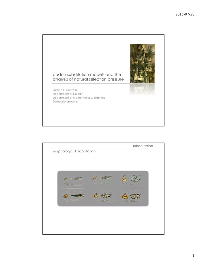
morphological adaptation introduction
2015-07-20 codon substitution models and the analysis of natural - - PDF document
2015-07-20 codon substitution models and the analysis of natural selection pressure Joseph P. Bielawski Department of Biology Department of Mathematics & Statistics Dalhousie University introduction morphological adaptation 1
2015-07-20 1 codon substitution models and the analysis of natural selection pressure
Joseph P. Bielawski Department of Biology Department of Mathematics & Statistics Dalhousie University
morphological adaptation introduction
2015-07-20 2
protein structure introduction
Troponin C: fast skeletal Troponin C: cardiac and slow skeletal
human cow rabbit rat
GTG CTG TCT CCT GCC GAC AAG ACC AAC GTC AAG GCC GCC TGG GGC AAG GTT GGC GCG CAC ... ... ... G.C ... ... ... T.. ..T ... ... ... ... ... ... ... ... ... .GC A.. ... ... ... ..C ..T ... ... ... ... A.. ... A.T ... ... .AA ... A.C ... AGC ... ... ..C ... G.A .AT ... ..A ... ... A.. ... AA. TG. ... ..G ... A.. ..T .GC ..T ... ..C ..G GA. ..T ... ... ..T C.. ..G ..A ... AT. ... ..T ... ..G ..A .GC ... GCT GGC GAG TAT GGT GCG GAG GCC CTG GAG AGG ATG TTC CTG TCC TTC CCC ACC ACC AAG ... ..A .CT ... ..C ..A ... ..T ... ... ... ... ... ... AG. ... ... ... ... ... .G. ... ... ... ..C ..C ... ... G.. ... ... ... ... T.. GG. ... ... ... ... ... .G. ..T ..A ... ..C .A. ... ... ..A C.. ... ... ... GCT G.. ... ... ... ... ... ..C ..T .CC ..C .CA ..T ..A ..T ..T .CC ..A .CC ... ..C ... ... ... ..T ... ..A ACC TAC TTC CCG CAC TTC GAC CTG AGC CAC GGC TCT GCC CAG GTT AAG GGC CAC GGC AAG ... ... ... ..C ... ... ... ... ... ... ... ..G ... ... ..C ... ... ... ... G.. ... ... ... ..C ... ... ... T.C .C. ... ... ... .AG ... A.C ..A .C. ... ... ... ... ... ... T.T ... A.T ..T G.A ... .C. ... ... ... ... ..C ... .CT ... ... ... ..T ... ... ..C ... ... ... ... TC. .C. ... ..C ... ... A.C C.. ..T ..T ..T ...
gene sequences introduction
2015-07-20 3
Powerful analytical tools: 1. Population genetic data 2. Comparative analysis of codon sequences 3. Comparative analysis of amino acid sequences
there is no single statistic which is best for testing the most general departures from neutrality
introduction
(Watterson 1977)
introduction
2015-07-20 4
1. introduction to the ω ratio 2. markov model of codon evolution 3. codon models for ω variation over branches & sites 4. model realism vs. model complexity
part I
http://www.langara.bc.ca/biology/mario/Assets/Geneticode.jpgpolypeptide
dS: number of synonymous
substitutions per synonymous site (KS)
dN: number of nonsynonymous
substitutions per nonsynonymous site (KA) ω : the ratio dN/dS; it measures selection at the protein level
Kimura (1968)
The genetic code determines how random changes to the gene brought about by the process of mutation will impact the function of the encoded protein.an index of natural selection pressure
2015-07-20 5
ω < 1 purifying (negative) selection histones ω =1 Neutral Evolution
pseudogenes
ω > 1 Diversifying (positive) selection MHC, Lysin rate ratio mode example
index of natural selection pressure: ω ratio
Why use dN and dS? (Why not use raw counts?)
Example of counts: 300 codon gene from a pair of species 5 synonymous differences 5 nonsynonymous differences 5/5 = 1 Why don’t we conclude that rates are equal (i.e., neutral evolution)? the basics
2015-07-20 6
Relative proportion of different types of mutations in hypothetical protein coding sequence.
Expected number of changes (proportion)
Type
All 3 Positions 1st positions 2nd positions 3rd positions
Total mutations
549 (100) 183 (100) 183 (100) 183 (100)
Synonymous
134 (25) 8 (4) (0) 126 (69)
Nonsyonymous
392 (71) 166 (91) 176 (96) 57 (27)
nonsense
23 (4) 9 (5) 7 (4) 7 (4)
Modified from Li and Graur (1991). Note that we assume a hypothetical model where all codons are used equally and that all types of point mutations are equally likely.
the basics
Why use dN and dS?
Same example, but using dN and dS: Synonymous sites = 25.5% S = 300 × 3 × 25.5% = 229.5 Nonsynonymous sites = 74.5% N = 300 × 3 × 74.5% = 670.5 So, dS = 5/229.5 = 0.0218 dN = 5/670.5 = 0.0075 dN/dS (ω) = 0.34, purifying selection !!! the basics
2015-07-20 7
Relative proportion of different types of mutations in hypothetical protein coding sequence.
Expected number of changes (proportion)
Type
All 3 Positions 1st positions 2nd positions 3rd positions
Total mutations
549 (100) 183 (100) 183 (100) 183 (100)
Synonymous
134 (25) 8 (4) (0) 126 (69)
Nonsyonymous
392 (71) 166 (91) 176 (96) 57 (27)
nonsense
23 (4) 9 (5) 7 (4) 7 (4)
Modified from Li and Graur (1991). Note that we assume a hypothetical model where all codons are used equally and that all types of point mutations are equally likely.
Note: by framing the counting of sites in this way we are using a “mutational opportunity” definition of the sites Not everyone agrees that this is the best approach. For an alternative view see Bierne and Eyre-Walker 2003 Genetics 168:1587-1597.
mutational opportunity
Partial codon usage table for the GstD gene of Drosophila
TTC 27 | TCC 15 | TAC 22 | TGC 6 Leu L TTA 0 | TCA 0 | *** * TAA 0 | *** * TGA 0 TTG 1 | TCG 1 | TAG 0 | Trp W TGG 8
CTC 2 | CCC 15 | CAC 4 | CGC 7 CTA 0 | CCA 3 | Gln Q CAA 0 | CGA 0 CTG 29 | CCG 1 | CAG 14 | CGG 0
real data have biases (Drosophila GstD1 gene)
preferred vs. un-preferred codons:
A G C T
ts/tv = 2.71
2015-07-20 8
Data from: Dunn, Bielawski, and Yang (2001) Genetics, 157: 295-305
1 2 3 4 0.4 0.8 1.2 1.6 2 2.4 2.8 t
d S
low codon bias 1 2 3 4 5 0.4 0.8 1.2 1.6 2 2.4 2.8 t
d S
extreme codon bias
true simple model ts/tv + codon bias
1 2 3 4 5 0.4 0.8 1.2 1.6 2 2.4 2.8 t
d S
high codon bias 1 2 3 4 0.4 0.8 1.2 1.6 2 2.4 2.8 t
d S
med codon bias
“corrections” and estimation bias in dS
Markov models of codon evolution
Goldman & Yang 1994 MBE 11:725-736 Muse & Gaut 1994 MBE 11:715-724
1. assumptions are explicit 2. “corrections” are not ad hoc 3. explicit use of a phylogeny improves power 4. principled framework for modelling and inference of the biology
x1 x2! x3 x4 j t1 t2 t0 t3 t4 kA G C T
2015-07-20 9 some important parameters:
“GY-style” codon models (mechanistic)
let’s model a change to CTG Synonymous CTC (Leu) CTG (Leu): πCTG
TTC (Leu) CTG (Leu): κπCTG
Nonsynonymous GTG (Val) CTG (Leu): ωπCTG
CCG (Pro) CTG (Leu): κωπCTG
→ → → →
“GY-style” codon models (mechanistic)
2015-07-20 10
to codon below: From codon below: TTT (Phe) TTC (Phe) TTA (Leu) TTG (Leu) CTT (Leu) CTC (Leu) GGG (Gly) TTT (Phe) −−− κπTTC ωπTTA ωπTTG ωκπTTT TTC (Phe) κπTTT −−− ωπTTA ωπTTG ωκπCTC TTA (Leu) ωπTTT ωπTTC −−− TTG (Leu) ωπTTT ωπTTC κπTTA −−− CTT (Leu) ωκπTTT −−− κπCTC CTC (Leu) ωκπTTC κπTTT −−− GGG (Gly) −−−
P(t) = {pij(t)} = eQt
* This is equivalent to the codon model of Goldman and Yang (1994). Parameter ω is the ratio dN/dS, κ is the transition/transversion rate ratio, and πi is the equilibrium frequency of the target codon (i).
“GY-style” codon models (mechanistic) P(t) = {pij(t)} = eQt
(Goldman & Yang 1994 MBE 11:725-736)
⎪ ⎪ ⎪ ⎩ ⎪ ⎪ ⎪ ⎨ ⎧ = n transitio nonsyn. for , ion transvers nonsyn. for , n transitio syn. for , ion transvers syn. for , positions 3
2 at differ and if
j j j j ij
j i q ωκπ ωπ κπ π
“GY-style” codon models (mechanistic)
2015-07-20 11
( ) ( )
1
) , ( t p t p CCT CCC L
kCCT kCCC k k h
π
∑
=
Note: analysis is typically done by using an unrooted tree
likelihood of the data at a site (only two codons) CCC
k
CCT
t1 t0
L = L1 × L2 × L3 × … × LN = ∏
= N 1 h h
L
ℓ = ln{L} = ln{L1} + ln{L2} + ln{L3} + … + ln{LN} =
∑
= N h h
L
1
} ln{
The likelihood of observing the entire sequence alignment is the product of the probabilities at each site.
The log likelihood is a sum over all sites.
likelihood of the data at all sites
2015-07-20 12
the good: we now have a framework for …
a new issue: averaging ω over a pair of sequences has very low power to detect positive selection if the question is about “when” or “where” ω > 1! we made some progress …
* Computation of transition probabilities accomplishes, in just one step, (1) a proper correction for multiple substitutions, (2) weighting for alternative pathways between codons and (3) is the basis for estimating the values of the model parameters from the data in hand.
Our question: When?
selection pressure (ω) varies in time
ε γG γA δ β 40 – 80 mya 150 – 200 mya 100 – 140 mya 35 mya
β globin gene cluster
2015-07-20 13
b.l. (my) Fraction of t ω
115 0.203 0.2 55 0.097 0.2 60 0.106 0.2 60 0.106 0.2 85 0.150 0.5 35 0.062 0.5 35 0.062 0.5 120 0.212 1.2
(Tot = 565my) (Tot = 1)
If we average over the tree, we do NOT detect positive selection; ω = 0.49.
Grey branches: ω = 0.2 Black branches: ω = 0.5 Blue branches: ω = 1.2
selection pressure (ω) varies in time
ε γG γA δ β 40 – 80 mya 150 – 200 mya 100 – 140 mya 35 myaselection pressure (ω) varies among sites
Our question: Where?
2015-07-20 14
ATG … … … … … … … … … … … … … … … … … … … … … … … … … … … … … … … … … … … . … … … … … … … … … … … … … … … … … … … … … … TAAIf we average over sites, we do NOT detect positive selection; ω = 0.31
selection pressure (ω) varies among sites
Purifying: dN/dS = 0.01 Neutral: dN/dS = 1 Adaptive: dN/dS = 2
problem: averaging ω over a pair has very low power if the questions are about “when” or “where”! solution: phylogenetic estimation of selection pressure
x1 x2! x3 x4 j
t1 t2 t0 t3 t4
k
likelihood of a phylogeny
2015-07-20 15
[ ]
∑∑
=
k j jx jx kj kx kx k h
t p t p t p t p t p x L ) ( ) ( ) ( ) ( ) ( ) (
1 2 3 4
1 2 3 4
π
x2 x4 x3 x1 t1 t2 t0 t3 t4 x1 x2 x3 x4 j
t1 t2 t0 t3 t4
Sum over all possible codons at ancestral nodes {TTT, TTC, …, GGG}
likelihood of a phylogeny k
improvements ….
x1 x2 x3
x4j t4:ω0 k t3:ω0 t0:ω0 t1:ω1 t2:ω1
GTG CTG TCT CCT GCC GAC AAG ACC AAC GTC AAG GCC GCC TGG GGC AAG GTT GGC GCG CAC ... ... ... G.C ... ... ... T.. ..T ... ... ... ... ... ... ... ... ... .GC A.. ... ... ... ..C ..T ... ... ... ... A.. ... A.T ... ... .AA ... A.C ... AGC ... ... ..C ... G.A .AT ... ..A ... ... A.. ... AA. TG. ... ..G ... A.. ..T .GC ..T ... ..C ..G GA. ..T ... ... ..T C.. ..G ..A ... AT. ... ..T ... ..G ..A .GC ...ω1 ω1 ω1 ω0 ω0
3.2. site models (ω varies among sites) 3.1. branch models (ω varies among branches)
2015-07-20 16
* These methods can be useful when selection pressure is strongly episodic
3.1. branch models *
x1 x2 x3
x4j t4:ω0 k t3:ω0 t0:ω0 t1:ω1 t2:ω1
Variation (ω) among branches: Approach Yang, 1998 fixed effects Bielawski and Yang, 2003 fixed effects Seo et al. 2004 auto-correlated rates Kosakovsky Pond and Frost, 2005 genetic algorithm Dutheil et al. 2012 clustering algorithm
3.1. branch models
x1 x2 x3
x4j t4:ω0 k t3:ω0 t0:ω0 t1:ω1 t2:ω1
2015-07-20 17
3.2. site models *
GTG CTG TCT CCT GCC GAC AAG ACC AAC GTC AAG GCC GCC TGG GGC AAG GTT GGC GCG CAC ... ... ... G.C ... ... ... T.. ..T ... ... ... ... ... ... ... ... ... .GC A.. ... ... ... ..C ..T ... ... ... ... A.. ... A.T ... ... .AA ... A.C ... AGC ... ... ..C ... G.A .AT ... ..A ... ... A.. ... AA. TG. ... ..G ... A.. ..T .GC ..T ... ..C ..G GA. ..T ... ... ..T C.. ..G ..A ... AT. ... ..T ... ..G ..A .GC ...Variation (ω) among sites: Approach Yang and Swanson, 2002 fixed effects (ML) Bao, Gu and Bielawski, 2006 fixed effects (ML) Massingham and Goldman, 2005 site wise (LRT) Kosakovsky Pond and Frost, 2005 site wise (LRT) Nielsen and Yang, 1998 mixture model (ML) Kosakovsky Pond, Frost and Muse, 2005 mixture model (ML) Huelsenbeck and Dyer, 2004; Huelsenbeck et al. 2006 mixture (Bayesian) Rubenstein et al. 2011 mixture model (ML) Bao, Gu, Dunn and Bielawski 2008 & 2011 mixture (LiBaC/MBC) Murell et al. 2013 mixture (Bayesian)
3.2. site models: “M-series”
Model Code NP Parameters One-ratio M0 1 ω Neutral M1a 2 P0, ω0, Selection M2a 4 p0, p1, ω0, ω2 Discrete M3 2K-1 p0, p1, ..., pK-2 ω0, ω1, …, ω K-2 Frequency M4 5 p0, p1, ..., p4 Gamma M5 2 α, β 2Gamma M6 4 p0, α0, β0, α1 Beta M7 2 p, q Beta&ω M8 4 p0, p, q, ω Beta&gamma M9 5 p0, p, q, α, β Beta&normal+1 M10 5 p0, p, q, α, β Beta&normal>1 M11 5 p0, p, q, μ, α 0&2normal>1 M12 5 p0, p1, μ2, α1, α2 3normal>0 M13 6 p0, p1, μ2, α0, α1, α2
2015-07-20 18
0.1 0.2 0.3 0.4 0.5 0.6 0.7 0.8 0.9 1= 0.01 = 1.0 = 2.0
ω ω ω
) | ( ) (
1 i h i K i h
P p P ω x x
∑
− =
=
3.2. discrete model
GTG CTG TCT CCT GCC GAC AAG ACC AAC GTC AAG GCC GCC TGG GGC AAG GTT GGC GCG CAC ... ... ... G.C ... ... ... T.. ..T ... ... ... ... ... ... ... ... ... .GC A.. ... ... ... ..C ..T ... ... ... ... A.. ... A.T ... ... .AA ... A.C ... AGC ... ... ..C ... G.A .AT ... ..A ... ... A.. ... AA. TG. ... ..G ... A.. ..T .GC ..T ... ..C ..G GA. ..T ... ... ..T C.. ..G ..A ... AT. ... ..T ... ..G ..A .GC ...“globin model” 3.2. site models
GTG CTG TCT CCT GCC GAC AAG ACC AAC GTC AAG GCC GCC TGG GGC AAG GTT GGC GCG CAC ... ... ... G.C ... ... ... T.. ..T ... ... ... ... ... ... ... ... ... .GC A.. ... ... ... ..C ..T ... ... ... ... A.. ... A.T ... ... .AA ... A.C ... AGC ... ... ..C ... G.A .AT ... ..A ... ... A.. ... AA. TG. ... ..G ... A.. ..T .GC ..T ... ..C ..G GA. ..T ... ... ..T C.. ..G ..A ... AT. ... ..T ... ..G ..A .GC ...“MHC model” directional selection diversifying selection
Site models detect diversifying positive selection; absence of “signal” under a sites model does not mean changes in a protein did not have fitness consequences (Bielawski et al. 2004 PNAS 101: 14824–29 ) site models
2015-07-20 19
3.2. site models
GTG CTG TCT CCT GCC GAC AAG ACC AAC GTC AAG GCC GCC TGG GGC AAG GTT GGC GCG CAC ... ... ... G.C ... ... ... T.. ..T ... ... ... ... ... ... ... ... ... .GC A.. ... ... ... ..C ..T ... ... ... ... A.. ... A.T ... ... .AA ... A.C ... AGC ... ... ..C ... G.A .AT ... ..A ... ... A.. ... AA. TG. ... ..G ... A.. ..T .GC ..T ... ..C ..G GA. ..T ... ... ..T C.. ..G ..A ... AT. ... ..T ... ..G ..A .GC ...we made some more progress ….
x1 x2 x3
x4j t4:ω0 k t3:ω0 t0:ω0 t1:ω1 t2:ω1
GTG CTG TCT CCT GCC GAC AAG ACC AAC GTC AAG GCC GCC TGG GGC AAG GTT GGC GCG CAC ... ... ... G.C ... ... ... T.. ..T ... ... ... ... ... ... ... ... ... .GC A.. ... ... ... ..C ..T ... ... ... ... A.. ... A.T ... ... .AA ... A.C ... AGC ... ... ..C ... G.A .AT ... ..A ... ... A.. ... AA. TG. ... ..G ... A.. ..T .GC ..T ... ..C ..G GA. ..T ... ... ..T C.. ..G ..A ... AT. ... ..T ... ..G ..A .GC ...ω1 ω1 ω1 ω0 ω0
3.2. site models (ω varies among sites) 3.1. branch models (ω varies among branches) 3.3. branch-site models (combines the features of above models)
2015-07-20 20
= 0.01 = 0.90 = 5.55
ω ω ω
Foreground branch only ω for background branches are from site-classes 1 and 2 (0.01 or 0.90)3.3. branch-site model: “model B”
) | ( ) (
1 i h i K i h
P p P ω x x
∑
− =
=
* These methods can be useful when selection pressures change over time at
just a fraction of sites
* It can be a challenge to apply these methods properly (more abut this later).
3.3. models for variation in branches & sites
Variation (ω) among branches & sites: Approach Yang and Nielsen, 2002 fixed+mixture (ML) Forsberg and Christiansen, 2003 fixed+mixture (ML) Bielawski and Yang, 2004 fixed+mixture (ML) Giundon et al., 2004 switching (ML) Zhang et al. 2005 fixed+mixture (ML) Kosakovsky Pond et al. 2011, 2012 full mixture (ML)
2015-07-20 21
(images from Paul Lewis)
simplification of a complex situation designed to eliminate extraneous detail in order to focus attention on the essentials of the situation
(Daniel L. Hartl)
total ¡error ¡ variance ¡
(high) ¡
model ¡complexity ¡
(low) ¡
total ¡error ¡ bias ¡
error ¡
there is a kind of “tension” between model realism and model complexity
“OVER FIT” “UNDER FIT”
2015-07-20 22
AA exchangeabilties
intentional simplification: all of the models listed above treat these two amino acid substitutions in the same way!
to codon below: From codon below: TTT (Phe) TTC (Phe) TTA (Leu) TTG (Leu) CTT (Leu) CTC (Leu) GGG (Gly) TTT (Phe) −−− κπTTC ωπTTA ωπTTG ωκπTTT TTC (Phe) κπTTT −−− ωπTTA ωπTTG ωκπCTC TTA (Leu) ωπTTT ωπTTC −−− TTG (Leu) ωπTTT ωπTTC κπTTA −−− CTT (Leu) ωκπTTT −−− κπCTC CTC (Leu) ωκπTTC κπTTT −−− GGG (Gly) −−−
* This is equivalent to the codon model of Goldman and Yang (1994). Parameter ω is the ratio dN/dS, κ is the transition/transversion rate ratio, and πi is the equilibrium frequency of the target codon (i).
Q matrix for M0 codon models
2015-07-20 23
structure of rate matrix: GY-M0
Structure of a Q matrix (log scaled and binned) derived from M0 for Abolone sperm lysin
2 parameters (κ and ω)
too sparse?
structure of rate matrix: ECM
Structure of a Q matrix (log scaled and binned) derived ECM (Kosiol et al. 2007) for all sequences in the Pandit database
1830 parameters
way too many!
2015-07-20 24
total ¡error ¡ variance ¡
(high) ¡
model ¡complexity ¡
(low) ¡
total ¡error ¡ bias ¡
error ¡
“OVER FIT ?” “UNDER FIT ?” codon rate matrix
trying to find a balance
parameters : 2 (fitted) 23 (fitted) 1830 (not fitted) lnL (Lysin) : -4124.58
question: does this impact inference of positive selection? preliminary answer: sometimes (but, oftentimes no)
2015-07-20 25
modeling amino acid exchangeabilities
PCP: physiochemcially constrained parametric model MEP: mixed empirical and parametric model ECM: empirical codon model GPP: general purpose parametric model * models permitting double and triple changes among codons
multiple amino acid exhangeabilities: model type Yang and Goldman 1994; Yang et al. 1998; PCP Sanudiin et al. 2005; Wong et al. 2006 PCP Conant and Stadler (2009)
PCP
Kosiol et al. 2007; De Maio et al. 2012 ECM è MEP * Doron-Faigenboin & Pupko 2007 MEP * Miyazawa (2011) MEP (LCEP) * Zoller and Schneider (2012) MEP (LCEP) * Delport et al. 2010 GPP (GA) Zaheri, Dib and Salamin (2014) GPP * Bielawski et al. (in prep.) GPP *
different preferences (that’s OK)
DECISIONS. codon models lots of options …
no single method will be suitable for all situations