20. Line integrals Lets look more at line integrals. Lets suppose we - PDF document

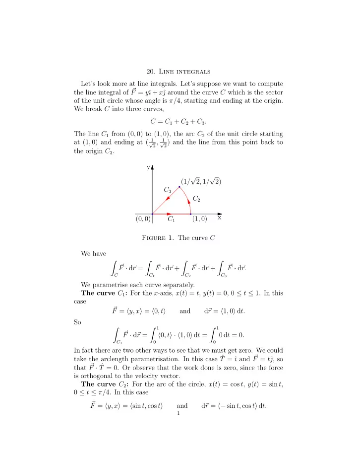
20. Line integrals Let’s look more at line integrals. Let’s suppose we want to compute the line integral of � F = y ˆ ı + x ˆ  around the curve C which is the sector of the unit circle whose angle is π/ 4, starting and ending at the origin. We break C into three curves, C = C 1 + C 2 + C 3 . The line C 1 from (0 , 0) to (1 , 0), the arc C 2 of the unit circle starting at (1 , 0) and ending at ( 1 1 2 , 2 ) and the line from this point back to √ √ the origin C 3 . y √ √ (1 / 2 , 1 / 2) C 3 C 2 x (0 , 0) (1 , 0) C 1 Figure 1. The curve C We have � � � � � � � � F · d � r = F · d � r + F · d � r + F · d � r. C C 1 C 2 C 3 We parametrise each curve separately. The curve C 1 : For the x -axis, x ( t ) = t , y ( t ) = 0, 0 ≤ t ≤ 1. In this case � F = � y, x � = � 0 , t � and d � r = � 1 , 0 � d t. So � 1 � 1 � � F · d � r = � 0 , t � · � 1 , 0 � d t = 0 d t = 0 . C 1 0 0 In fact there are two other ways to see that we must get zero. We could take the arclength parametrisation. In this case ˆ ı and � T = ˆ F = t ˆ  , so that � F · ˆ T = 0. Or observe that the work done is zero, since the force is orthogonal to the velocity vector. The curve C 2 : For the arc of the circle, x ( t ) = cos t , y ( t ) = sin t , 0 ≤ t ≤ π/ 4. In this case � F = � y, x � = � sin t, cos t � and d � r = �− sin t, cos t � d t. 1

So � π/ 4 � π/ 4 � π/ 4 � sin(2 t ) � = 1 � F · d � r = � sin t, cos t �·�− sin t, cos t � d t = cos(2 t ) d t = 2 . 2 C 2 0 0 0 The curve C 3 : For the straight line segment starting at ( 1 1 2 , 2 ) √ √ √ and ending at the origin, we have x ( t ) = t , y ( t ) = t , 0 ≤ t ≤ 1 / 2. � F = � y, x � = � t, t � and d � r = � 1 , 1 � d t. So, � 0 � 0 � 0 � = − 1 � � t 2 F · d � r = � t, t � · � 1 , 1 � d t = 2 t d t = 2 . √ √ C 3 1 / 1 / √ 2 2 1 / 2 √ Note that the limits start at 1 / 2 and end at 0. Putting all of this together, we get � � � � � � � � F · d � r = F · d � r + F · d � r + F · d � r = 0 + 1 / 2 − 1 / 2 = 0 . C C 1 C 2 C 3 We say that � F is a gradient field if � F = ∇ f , for some scalar function f . Theorem 20.1 (Fundamental Theorem of Calculus for line integrals) . If � F = ∇ f is a gradient vector field then � � � F · d � r = ∇ f · d � r = f ( P 1 ) − f ( P 0 ) , C C where C is a path from P 0 to P 1 . For example, suppose we take f ( x, y ) = xy . Then  = � ∇ f = y ˆ ı + x ˆ F, the vector field above. Using (20.1), we see that � � F · d � r = f (0 , 0) − f (0 , 0) = 0 . C On the other hand, r = f ( 1 2 , 1 2) − f (1 , 0) = 1 � � √ √ F · d � 2 . C 2 In the language of differentials, one can restate (20.1) as � � f x d x + f y d y = d f = f ( P 1 ) − f ( P 0 ) . C C 2

Proof of (20.1) . � t 1 � � dx dy � ∇ f · d � r = f x dt + f y d t dt C t 0 � t 1 d = dt ( f ( x ( t ) , y ( t ))) d t t 0 � t 1 � = f ( x ( t ) , y ( t )) t 0 = f ( P 1 ) − f ( P 0 ) . � (20.1) has some very interesting consequences: Path independence: If C 1 and C 2 are two paths starting and ending at the same point, then � � ∇ f · d � r = ∇ f · d � r. C 1 C 2 In other words, the line integral � ∇ f · d � r, C depends only on the endpoints, not on the trajectory. Gradient fields are conservative: If C is a closed loop, then � ∇ f · d � r = 0 . C We already saw that if C is a circle of radius a centred at the circle and � F = − y ˆ ı + x ˆ  , then � r = 2 πa 2 � = 0 . � F · d � C So the vector field � F = − y ˆ ı + x ˆ  is not conservative. It follows that � F = − y ˆ ı + x ˆ  is not the gradient of any scalar field. If � F = ∇ f is a gradient field, and � F is the force, then f has an interesting physical interpretation, it is called the potential. In this case the work done is nothing more than the change in the potential. For example, if � F is the force due to gravity, f is inversely proportional to the height. If � F is the electric field, f is the voltage. (Note the annoying fact that mathematicians and physicists use a different sign convention; for physicists � F = −∇ f ). To summarise, we have four equivalent properties: (1) � C � � F is conservative, that is, F · d � r = 0 for any closed loop. C � � (2) F · d � r is path independent. 3

(3) � F = ∇ f is a gradient vector field. (4) M d x + N d y is an exact differential, equal to d f . (1) and (2) are equivalent by considering the closed loop C = C 1 − C 2 . (3) implies (2) by (20.1). We will see (2) implies (3) in the next lecture. (3) and (4) are the same statement, using different notation. 4