15-11-2019 Department of Veterinary and Animal Sciences Department - PDF document

15-11-2019 Department of Veterinary and Animal Sciences Department of Veterinary and Animal Sciences Decision making in general When a decision is made concerning a unit, the following information is necessary: • The present state of the unit Linear programming • The relation between factors and production • Immediate production • Future production Anders Ringgaard Kristensen • The farmer’s personal preferences • All constraints of legal, economic, physical or personal kind Slide 2 Department of Veterinary and Animal Sciences Department of Veterinary and Animal Sciences Linear programming Example: Ration formulation Knowledge representation: A group of dairy cows is fed a ration consisting of x 1 kg silage • State of system: and x 2 kg concentrates. • Hidden in model formulation – often as constraints or as parameters The price of silage is p 1 and the price of concentrates is p 2 . • Factor/product relation: The ration must satisfy some nutritional “demands”: • Immediate production: • The energy content must be at least b 1 . • Linear function The AAT 1 value must be at least b 2 • Future production: • State of the cows • Static method The PBV 2 value must be at most b 3 • • Farmer preferences: • The fill must be at most b 4 • Linear utility function • Constraints: For both feeds, i , x i ≥ 0 • Linear constraints Determine x 1 and x 2 so that the cost of the ration is minimized. 1 AAT = Amino Acids absorbed in the intestine 2 PBV = Protein balance in the rumen Slide 3 Slide 4 Department of Veterinary and Animal Sciences What are the states of the feeds? 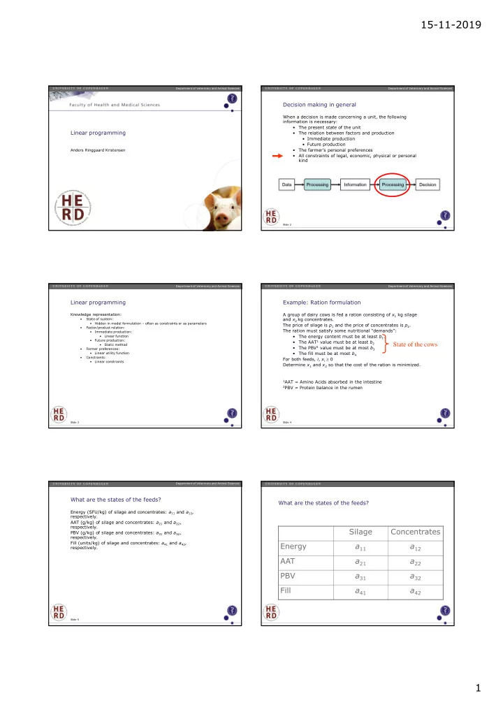What are the states of the feeds? Energy (SFU/kg) of silage and concentrates: a 11 and a 12 , respectively. AAT (g/kg) of silage and concentrates: a 21 and a 22 , respectively. Silage Concentrates PBV (g/kg) of silage and concentrates: a 31 and a 32 , respectively. Fill (units/kg) of silage and concentrates: a 41 and a 42 , Energy a 11 a 12 respectively. AAT a 21 a 22 PBV a 31 a 32 Fill a 41 a 42 Slide 5 1

15-11-2019 Department of Veterinary and Animal Sciences Department of Veterinary and Animal Sciences LP problem The linear relations: Two “activities” Objective function a 11 x 1 + a 12 x 2 ≥ b 1 ⇔ p 1 x 1 + p 2 x 2 = Min! (minimize costs) x 2 x 2 ≥ b 1 / a 12 – ( a 11 / a 12 ) x 1 - subject to b 1 / a 12 The permitted area is bounded a 11 x 1 + a 12 x 2 ≥ b 1 (energy at least b 1 ) by a straight line in the a 21 x 1 + a 22 x 2 ≥ b 2 (AAT at least b 2 ) diagram a 31 x 1 + a 32 x 2 ≤ b 3 (PBV at most b 3 ) a 41 x 1 + a 42 x 2 ≤ b 4 (fill at most b 4 ) x 1 x 1 ≥ 0, x 2 ≥ 0 Slope: a 11 / a 12 Constraints Slide 7 Slide 8 Department of Veterinary and Animal Sciences Graphical solution, convex area The objective function x 2 Energy, ≥ p 1 x 1 + p 2 x 2 = c (costs) AAT, ≥ PBV, ≤ Fill, ≤ For fixed cost c’ we have The per-mitted area x 2 = c’ / p 2 – ( p 1 / p 2 ) x 1 forms a convex set Combinations of x 1 and x 2 having same total cost form a straight line in the plane. x 1 Slide 10 Graphical solution, minimization Graphical solution, iso-cost line x 2 x 2 c’ / p 2 We want to minimize cost c’ Decrease c’ until the permitted area is reached. Decrease c’ until the lowest value of the permitted area is found. Optimal combination is x 1 ’, x 2 ’ Combinations of x 1 and x 2 having cost c’ Slope: p 1 / p 2 We want to minimize cost c’ x 2 ’ x 1 x 1 x 1 ’ 2

15-11-2019 Department of Veterinary and Animal Sciences What determines the optimum Influence of prices, I For a given set of constraints, the optimum is determined solely x 2 by the price relations. In our two-dimensional example it is simply the price ratio Original setting p 1 / p 2 Illustration x 2 ’ x 1 Slide 13 x 1 ’ Influence of prices, II Influence of prices, III x 2 x 2 Slight increase of p 1 Large increase of p 2 Drastic change in terms of x 1 and x 2 Drastic change in terms of x 1 and x 2 but only sligtly in terms of costs c and to some extent c x 2 ’ x 2 ’ x 1 x 1 x 1 ’ x 1 ’ Department of Veterinary and Animal Sciences Properties of linear programming Non-unique optimum The permitted area is always a convex set x 2 The optimal solution is: • Either uniquely located in a corner Increase of p 2 All combinations of x 1 and x 2 along a • Or along a border line (accordingly also in two corners) border are optimal It is therefore sufficient to search the corners of the convex set. A convex set A non-convex set x 1 Slide 18 3

15-11-2019 Department of Veterinary and Animal Sciences Department of Veterinary and Animal Sciences Modeling tricks More than two variables We cannot illustrate graphically anymore, but the same principles apply: From maximization to minimization: • Convex (multi-dimensional) set • p 1 x 1 + p 2 x 2 = Max! ⇔ - p 1 x 1 - p 2 x 2 = Min! • Optimum always in a corner From greater than to less than: • a i 1 x 1 + a i 2 x 2 ≥ b i ⇔ - a i 1 x 1 - a i 2 x 2 ≤ - b i From “equal to” to “less than” • a i 1 x 1 + a i 2 x 2 = b i ⇔ • - a i 1 x 1 - a i 2 x 2 ≤ - b i • a i 1 x 1 + a i 2 x 2 ≤ b i Slide 19 Slide 20 Department of Veterinary and Animal Sciences Department of Veterinary and Animal Sciences The simplex algorithm Shadow prices The most commonly applied optimization algorithm for linear What is the economic benefit of relaxing a constraint by one programming. unit? The simplex algorithm: • If it is not limiting it is zero! • Identifies a corner of the convex set forming the permitted area. • Trivial method: • Searches along the edges to find a better corner. • Change the constraint by one • Checks whether the present corner is optimal Implemented in modern standard spreadsheets • Optimize again Implemented in ration formulation programs • How much did the result improve? • Software systems typically provides these values by default. Slide 21 Slide 22 Department of Veterinary and Animal Sciences Basic assumptions of LP McCull and his sheep & steers Proportionality McCull owns 200 ha of pasture • No start-up costs where he can have ewes and/or Carrying capacity • No decreasing returns to scale steers. Additivity Gross margins are $24 per ewe and Season Ewes Steers • No interactions between activities $60 per steer. Divisibility Limited carrying capacity – refer to • Any proportion of an activity allowed table Spring 15 5 Certainty • All parameters (coefficients, prices, constraints) are known precisely. Summer 24 4 Autumn 15 Winter 8 Slide 23 4

15-11-2019 Department of Veterinary and Animal Sciences McCull: LP-problem McCull: Graphical solution Objective function: 5000 24 x 1 + 60 x 2 = Max! 4500 4000 Constraints: 3500 1/15 x 1 + 1/5 x 2 ≤ 200 3000 Spring grazing 1/24 x 1 + 1/4 x 2 ≤ 200 2500 Summer grazing x 1 ≤ 3000 (i.e 15 x 200) 2000 Sheep in autumn 1500 x 1 ≤ 1600 (i.e 8 x 200) Sheep in winter 1000 500 x 1 ≥ 0, x 2 ≥ 0 0 0 200 400 600 800 1000 Spring grazing Summer grazing Sheep in autumn Sheep in winter Iso-cost Slide 26 Department of Veterinary and Animal Sciences Properties of methods for decision support Herd constraints Optimization Linear programming Biological Functional variation limitations Slide 27 Uncertainty Dynamics 5