14/04/2016 Global vs Partitioned scheduling Single shared queue - - PDF document

SLIDE 1

14/04/2016 1

1

Global Scheduling in Multiprocessor Real-Time Systems

Alessandra Melani

2

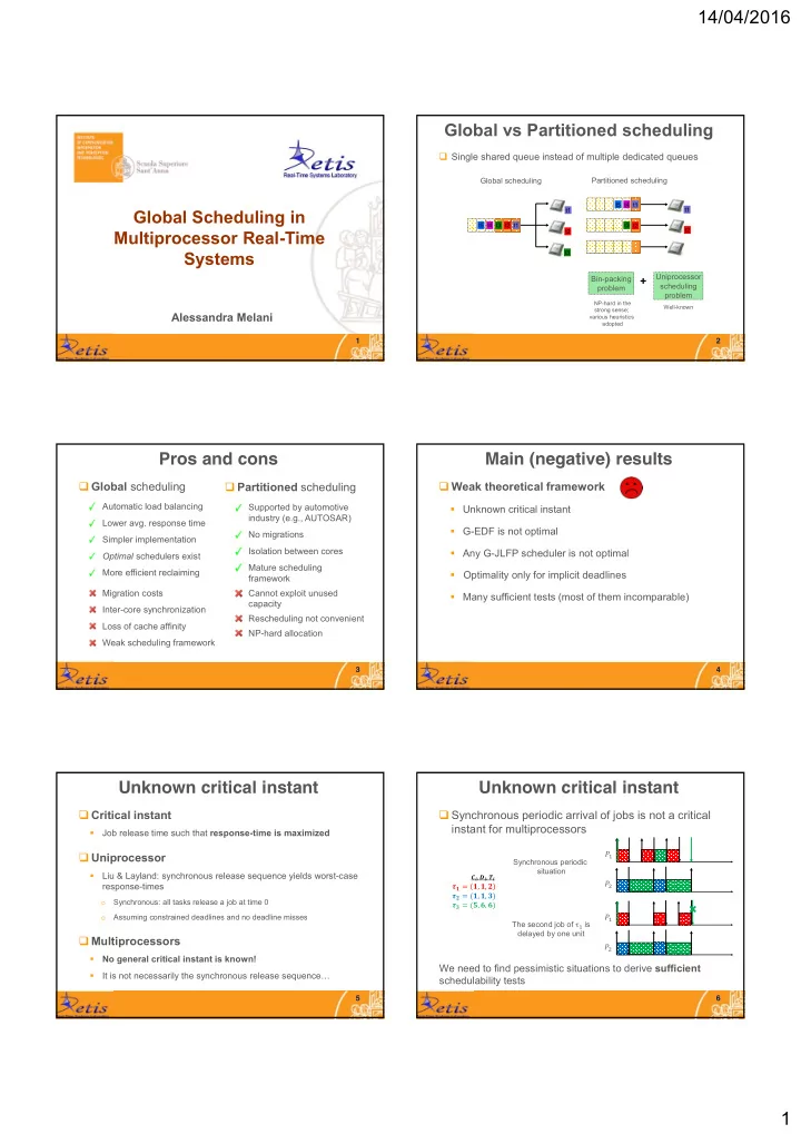
Global vs Partitioned scheduling

 Single shared queue instead of multiple dedicated queues

Bin-packing problem Uniprocessor scheduling problem

+

NP-hard in the strong sense; various heuristics adopted Well-known t2 t1 t3 t4 t5 t3 t1 t4 t5 t2

Global scheduling Partitioned scheduling

t1 t2 t3 t1 t2

3

Pros and cons

 Global scheduling

Automatic load balancing Lower avg. response time Simpler implementation Optimal schedulers exist More efficient reclaiming Migration costs Inter-core synchronization Loss of cache affinity Weak scheduling framework

 Partitioned scheduling

Supported by automotive industry (e.g., AUTOSAR) No migrations Isolation between cores Mature scheduling framework Cannot exploit unused capacity Rescheduling not convenient NP-hard allocation

4

Main (negative) results

 Weak theoretical framework

• Unknown critical instant
• G-EDF is not optimal
• Any G-JLFP scheduler is not optimal
• Optimality only for implicit deadlines
• Many sufficient tests (most of them incomparable)

5

Unknown critical instant

 Critical instant

• Job release time such that response-time is maximized

 Uniprocessor

• Liu & Layland: synchronous release sequence yields worst-case

response-times

• Synchronous: all tasks release a job at time 0
• Assuming constrained deadlines and no deadline misses

 Multiprocessors

• No general critical instant is known!
• It is not necessarily the synchronous release sequence…

6

Unknown critical instant

 Synchronous periodic arrival of jobs is not a critical instant for multiprocessors

Synchronous periodic situation The second job of τ is delayed by one unit

We need to find pessimistic situations to derive sufficient schedulability tests

, , , , , ,

• , ,

SLIDE 2

14/04/2016 2

7

G-EDF is not optimal

 Uniprocessors

• EDF is optimal

 Multiprocessors

• G-EDF is not optimal
• Key problem: sequentiality of tasks
• Two processors available for τ,

but it can only use one

τ τ τ τ τ

Scheduled on processor 1 Scheduled on processor 2 8

Any G-JLFP scheduler is not optimal

Two processors, three tasks, 15, 10  Any job-level fixed-priority scheduler is not optimal

• Synchronous release time
• One of the three jobs is scheduled last under any JLFP policy
• Deadline miss unavoidable!

τ τ τ

Scheduled on processor 1 Scheduled on processor 2 9

G-JLDP required for optimality

Job priority changes!

τ τ τ

Scheduled on processor 1 Scheduled on processor 2

τ τ τ

Scheduled on processor 1 Scheduled on processor 2

G-JLFP G-JLDP

 G-JLDP: Global Job Level Dynamic Priority; the priority of each job may change over time

10

Taxonomy of multiprocessor scheduling algorithms

Uniprocessor Algorithms

LLF EDF

Partitioned Algorithms Global Algorithms

Global EDF

Dedicated Global Algorithms

Partitioned EDF

Optimal Algorithms

EKG DP-Wrap pfair LLREF

Uniprocessor Multiprocessor

RM Partitioned FP Global FP DM

Optimal Not

• ptimal

anymore 11

Proportionate fairness

 P-fair: notion of “fair share of processor”  If a schedule is P-fair, no implicit deadline will be missed →

• ptimal algorithm

Basic principle:  Timeline is divided into equal length slots  Task period and execution time are multiples of the slot size  Each task receives amount of slots proportional to its task utilization

• If a task has utilization
• , then it will have been allocated ∙ time slots

for execution in the interval 0, 12

Proportionate fairness

Example:

 3;

6

•  Quantum-based: ∈ , ∈ ; scheduling decisions can only occur

at integers  A task executes during a whole time slot or not execute at all in that time slot

τ τ

SLIDE 3

14/04/2016 3

13

Proportionate fairness

τ, ∙

• τ,

 Goal: find an algorithm that minimizes max

• |τ, |

 Which are the values that can take? Error “Fluid” execution: should have executed in 0, Real execution in 0,

14

 Example: τ

• 5, 2 ,

7, 4 , 1 processor

Proportionate fairness

τ τ τ τ τ τ

No task executes in 0,1 τ, 1 1 ∙

• 0 0

τ, 1 1 ∙

• 0 0

Task τ executes in 0,1 τ, 1 1 ∙

• 1 0

τ, 1 1 ∙

• 0 0

Task τ executes in 0,1 τ, 1 1 ∙

• 0 0

τ, 1 1 ∙

• 1 0

τ, 1 0 is impossible

15

Proportionate fairness

 Example: τ

• 4, 1 ,
• 4, 1 ,

4, 1 , 4, 1

,

• ne processor

τ, 1 1 ∙ 1 4 1 3 4 τ, 3 3 ∙ 1 4 0 3 4

τ τ τ τ

1 τ, 1 seems to be the worst-case lag

16

 Definition (P-fair schedule): a schedule is P-fair if and only if ∀ τ and ∀ : 1 τ, 1 / 1

Execution domain of P-fair

• τ,

Slope

Proportionate fairness

17

Proportionate fairness

 Theorem A P-fair schedule is optimal in the sense of feasibility for a set of periodic tasks with implicit deadlines  Proof A schedule is P-fair ⇒ 1 τ, 1 ⇒ 1 τ, 1 ⇒ 1

• τ, 1

⇒ 1 τ, 1 ⇒ τ, 0 ⇒ τ, 1 τ, ⇒ τ, ⇒ τ executes time-units during , 1 ⇒ τ meets every deadline in periodic scheduling

18

The algorithm PF

 How to generate a P-fair schedule?

• Execute all urgent tasks
• A task τ is urgent at time if

τ, 0 and τ, 1 0 if τ executes

• Do not execute tnegru tasks
• A task τ is tnegru at time if

τ, 0 and τ, 1 0 if τ does not execute

• For the other tasks, execute the task that has the least such

that τ, 0

SLIDE 4

14/04/2016 4

19

The algorithm PF

 Results

• The algorithm PF assigns priorities to tasks at every time slot →

Job-level dynamic priority (JLDP) scheduling policy

• Theorem: the schedule generated by algorithm PF is P-fair
• Proof: [Baruah et al., ‘96]

20

The algorithm PF

 Example: τ

• 5, 2 ,

5, 3 , one

processor

τ

At time 1: τ, 1 1 ∙ 2 5 1 3 5 τ, 1 1 ∙ 3 5 0 3 5 At time 0, any of the two tasks may be scheduled At time 2 if τ executes: τ, 2 2 ∙ 3 5 1 1 5 τ is urgent at time 1!! 21

The algorithm PF

 Example: τ

• 5, 2 ,

5, 3 , one

processor

τ

At time 2: τ, 2 2 ∙ 2 5 1 1 5 τ, 2 2 ∙ 3 5 1 1 5 At time 3 if τ executes: τ, 3 3 ∙ 2 5 1 1 5 τ, 3 3 ∙ 3 5 2 1 5 τ is scheduled since it has the least such that lag is positive 22

The algorithm PF

 Example: τ

• 5, 2 ,

5, 3 , one

processor

τ

At time 3: τ, 3 3 ∙ 2 5 1 1 5 τ, 3 3 ∙ 3 5 2 1 5 At time 4 if τ executes: τ, 4 4 ∙ 2 5 2 2 5 τ is scheduled since it has the least such that lag is positive 23

The algorithm PF

 Example: τ

• 5, 2 ,

5, 3 , one

processor

τ

At time 4: τ, 4 4 ∙ 2 5 2 2 5 τ, 4 4 ∙ 3 5 2 2 5 At time 5 if τ executes: τ, 5 5 ∙ 3 5 3 0 τ is urgent at time 4!!

…and so on…

24

Proportionate fairness

 Exact test of existence of a P-fair schedule:

•  Full processor utilization!

Disadvantages

 High number of preemptions  High number of migrations  Optimal only for implicit deadlines

SLIDE 5

14/04/2016 5

25

(Other) negative results

 No optimal algorithm is known for constrained or arbitrary deadline systems  No optimal online algorithm is possible for arbitrary collections of jobs [Leung and Whitehead]  Even for sporadic task systems, optimality requires clairvoyance [Fisher et al., 2009] ⇒ Many sufficient schedulability tests exist, according to different metrics of evaluation

 Percentage of schedulable task-sets detected ⟹ RTA-based test

26

 Response time analysis

• In a uniprocessor system, it provides a necessary and sufficient

test for fixed-priority preemptive scheduling with constrained deadlines

• In a multiprocessor system, it provides an only sufficient

schedulability test

• How to compute interference from higher-priority tasks?

RTA-based test

Exact interference from higher- priority tasks

27

Introducing the interference

k

Task under analysis

τi

Interference of τ on τ

τi τ3 τ1 τ2 τ5 τ2 τ3 τi τi τ3 τ6 τ5 τ4 τ7 τ8

ri ri + Ri

m

Global FP and Global EDF are work-conserving schedulers Work-conserving scheduler: it never idles a core if there is workload ready to be executed

1 ,

• 28

Introducing the interference

k

Task under analysis

τi

Interference of τ on τ

1

• τi

τ3 τ1 τ2 τ5 τ2 τ3 τi τi τ3 τ6 τ5 τ4 τ7 τ8

ri ri + Ri

m

For work-conserving schedulers: a ready job cannot execute

• nly if all m

processors are busy We can safely assume that the interference is distributed across all m processors

1 ,

• 29

Limiting the interference

1 min

• , 1
• It is sufficient to consider at most the portion 1 of each

term

in the sum

It can be proved that is given by the fixed point iteration of:

k

Task under analysis

τi

Interference of τ on τ

τi τ3 τ1 τ2 τ5 τ2 τ3 τi τi τ3 τ6 τ5 τ4 τ7 τ8

ri ri + Ri

m 30

Bounding the interference

•  Exactly computing the interference is complex
• No critical instant scenario

 Pessimistic assumptions:

• 1. Bound the interference of a task with the workload
• 2. Use an upper-bound to the workload

SLIDE 6

14/04/2016 6

31

Bounding the workload

Consider a pessimistic situation in which:

• The first job executes as close as possible to its deadline
• Successive jobs execute as soon as possible

Ck k



L Dk

Ck Ck Ck

Tk εk

• ∙

Where:

• ε min

, ∙

Number of jobs excluding the last one Last job 32

RTA for generic global schedulers

An upper-bound on the worst-case response time of is given by the fixed point iteration of:

← 1 min , 1

• The slack of is at least:

Ri Si 33

Improvement using slack values

Consider a pessimistic situation in which:

• The first job executes as close as possible to its deadline
• Successive jobs execute as soon as possible

Ck k



L Dk

Ck Ck Ck

Tk Sk

• , , ∙ ,

Where: ,

• ε , min

, , ∙

Number of jobs excluding the last one Last job 34

Improvement using slack values

• , , ∙ ,

Where: ,

• ε , min

, , ∙

Number of jobs excluding the last one Last job

Ck k



L Dk

Ck Ck Ck

Tk Rk

Consider a pessimistic situation in which:

• The first job executes as close as possible to its deadline
• Successive jobs execute as soon as possible

35

RTA for generic global schedulers

An upper-bound on the worst-case response time of is given by the fixed point iteration of:

← 1 min , , 1

• If a fixed point is reached for every task in the system,

the task set is schedulable with any work-conserving global scheduler

36

Iterative schedulability test

• 1. All response times initialized to
• 2. Compute response time bound for tasks 1, … ,
• If larger than old value ⟶ update
• If , mark as temporarily not schedulable
• 3. If no response time has been updated for tasks 1, … , and

all tasks have ⟶ return success

• 4. If no response time has been updated for tasks 1, … , and

for some task ⟶ return fail

• 5. Otherwise, return to point 2

SLIDE 7

14/04/2016 7

37

RTA refinement for Fixed Priority

 The interference from lower priority tasks is always null

• 0, ∀

 An upper bound on the worst-case response time of can be given by the fixed point iteration of

← 1 min , , 1

• 38

RTA refinement for EDF

 A different bound can be derived analyzing the worst-case workload in a situation in which:

• The interfering and interfered tasks have a common

deadline

• All jobs execute as late as possible
• ′,

Ck k



Dk

Ck Ck Ck

Tk Rk

i



Di 39

RTA refinement for EDF

 An upper-bound on the worst-case response time of is given by the fixed point iteration of

• ,
• min ,
• Ck

k



Dk

Ck Ck Ck

Tk Rk

i



Di

← 1 min , , 1,

,

• Sk

40

Complexity

 Pseudo-polynomial complexity  Fast average behavior  Lower complexity for Fixed Priority systems

• Response times are updated in decreasing priority order

 Multiple rounds may be needed in the general case

41

Thank you!

Alessandra Melani alessandra.melani@sssup.it