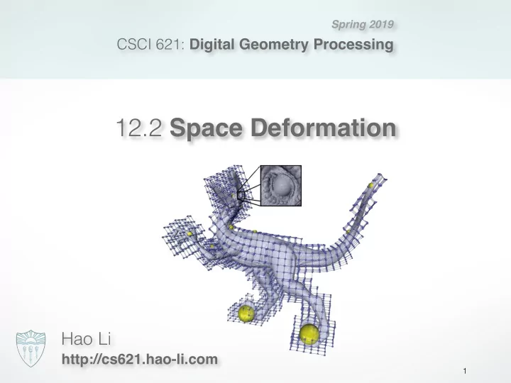
12.2 Space Deformation Hao Li http://cs621.hao-li.com 1 Hoooray! - PowerPoint PPT Presentation

Spring 2019 CSCI 621: Digital Geometry Processing 12.2 Space Deformation Hao Li http://cs621.hao-li.com 1

Hoooray! 2

Last Time Surface Deformations 3

Space Deformation ● Displacement function defined on the ambient space d : R 3 → R 3 ● Evaluate the function on the points of the shape embedded in the space x 0 = x + d ( x ) Twist warp Global and local deformation of solids [A. Barr, SIGGRAPH 84] 4

Freeform Deformation ● Control object ● User defines displacements d i for each element of the control object ● Displacements are interpolated to the entire B i ( x ) : R 3 → R space using basis functions k X d ( x ) = d i B i ( x ) i =1 ● Basis functions should be smooth for aesthetic results 5

Freeform Deformation [Sederberg & Parry 86] ● Control object = lattice ● Basis functions B i ( x ) are trivariate tensor-product splines: l m n X X X d ( x, y, z ) = d ijk N i ( x ) N j ( y ) N k ( z ) i =0 j =0 k =0 6

Freeform Deformation [Sederberg & Parry 86] ● Aliasing artifacts ● Interpolate deformation constraints? ! Only in least squares sense 7

Limitations of Lattices as Control Objects ● Difficult to manipulate ● The control object is not related to the shape of the edited object ● Parts of the shape in close Euclidean distance always deform similarly, even if geodesically far 8

Wires [Singh & Fiume 98] ● Control objects are arbitrary space curves ● Can place curves along meaningful features of the edited object ● Smooth deformations around the curve with decreasing influence 9

Handle Metaphor [RBF, Botsch & Kobbelt 05] ● Wish list for the displacement function d ( x ) : ! Interpolate prescribed constraints ! Smooth, intuitive deformation d ( x i ) = d i d : R 3 → R 3 x → x + d ( x ) 10

Volumetric Energy Minimization [RBF, Botsch & Kobbelt 05] ● Minimize similar energies to surface case Z R 3 k d xx k 2 + k d xy k 2 + . . . + k d zz k 2 dx dy dz ! min ● But displacements function lives in 3D... ! Need a volumetric space tessellation? ! No, same functionality provided by RBFs! 11

Radial Basis Functions [RBF, Botsch & Kobbelt 05] ● Represent deformation by RBFs X d ( x ) = w j ϕ ( k c j � x k ) + p ( x ) j ● Triharmonic basis function ϕ ( r ) = r 3 ! C 2 boundary constraints ! Highly smooth / fair interpolation Z R 3 k d xxx k 2 + k d xyy k 2 + . . . + k d zzz k 2 dx dy dz ! min 12

Radial Basis Functions [RBF, Botsch & Kobbelt 05] ● Represent deformation by RBFs X d ( x ) = w j ϕ ( k c j � x k ) + p ( x ) j ● RBF fitting ! Interpolate displacement constraints ! Solve linear system for w j and p ! 13

Radial Basis Functions [RBF, Botsch & Kobbelt 05] ● Represent deformation by RBFs X d ( x ) = w j ϕ ( k c j � x k ) + p ( x ) j ● RBF evaluation ! Function d transforms points ! Jacobian ∇ d transforms normals ! Precompute basis functions ! ! Evaluate on the GPU! 14

Local & Global Deformations [RBF, Botsch & Kobbelt 05] 15

Local & Global Deformations [RBF, Botsch & Kobbelt 05] 1M vertices movie 16

Space Deformation ● Handle arbitrary input ! Meshes (also non-manifold) ! Point sets ! Polygonal soups ! … ! 3M triangles ● Complexity mainly depends ! 10k components ! Not oriented on the control object, not ! Not manifold the surface 17

Space Deformation ● Handle arbitrary input ! Meshes (also non-manifold) ! Point sets ! Polygonal soups ! … ● Easier to analyze: functions on Euclidean domain ! Volume preservation: |Jacobian| = 1 18

Space Deformation ● The deformation is only loosely aware of the shape that is being edited ● Small Euclidean distance → similar deformation ● Local surface detail may be distorted 19

Cage-Based Deformation [Ju et al. 05] ● Cage = crude version of the input shape ● Polytope (not a lattice) 20

Cage-Based Deformation [Ju et al. 05] ● Each point x in space is represented w.r.t. to the cage elements using coordinate functions k v x p i X x = w i ( x ) p i i =1 21

Cage-Based Deformation [Ju et al. 05] ● Each point x in space is represented w.r.t. to the cage elements using coordinate functions k x p i X x = w i ( x ) p i i =1 22

Cage-Based Deformation [Ju et al. 05] k x 0 = X w i ( x ) p 0 i x ! i =1 p ! i x p i 23

Generalized Barycentric Coordinates ● Lagrange property: w i ( p j ) = δ ij k X ● Reproduction: w i ( x ) p i = x ∀ x , i =1 k X ● Partition of unity: w i ( x ) = 1 ∀ x , i =1 24

Coordinate Functions ● Mean-value coordinates [Floater 2003, Ju et al. 2005] ! Generalization of barycentric coordinates ! Closed-form solution for w i ( x ) 25

Coordinate Functions ● Mean-value coordinates [Floater, Ju et al. 2005] ! Not necessarily positive on non-convex domains 26

Coordinate Functions ● Harmonic coordinates (Joshi et al. 2007) ! Harmonic functions h i ( x ) for each cage vertex p i Δ h = 0 ! Solve subject to: h i linear on the boundary s.t. h i ( p j ) = δ ij MVC HC 27

Coordinate Functions ● Harmonic coordinates (Joshi et al. 2007) ! Harmonic functions h i ( x ) for each cage vertex p i Δ h = 0 ! Solve subject to: h i linear on the boundary s.t. h i ( p j ) = δ ij ● Volumetric Laplace equation ● Discretization, no closed-form 28

Coordinate Functions ● Harmonic coordinates (Joshi et al. 2007) MVC HC 29

Coordinate Functions ● Green coordinates (Lipman et al. 2008) ● Observation: previous vertex-based basis functions always lead to affine- invariance! k m x 0 = X X w i ( x ) p 0 ψ j ( x ) n 0 i + j i =1 j =1 30

Coordinate Functions ● Green coordinates (Lipman et al. 2008) ● Correction: Make the coordinates depend on the cage faces as well k m x 0 = X X w i ( x ) p 0 ψ j ( x ) n 0 i + j i =1 j =1 31

Coordinate Functions ● Green coordinates (Lipman et al. 2008) ● Closed-form solution ● Conformal in 2D, quasi-conformal in 3D GC MVC GC 32

Coordinate Functions ● Green coordinates (Lipman et al. 2008) ● Closed-form solution ● Conformal in 2D, quasi-conformal in 3D Alternative interpretation in 2D via holomorphic functions and extension to point handles : Weber et al. Eurographics 2009 33

Cage-Based Methods: Summary Pros: ● Nice control over volume ! Squish/stretch Cons: ● Hard to control details of embedded surface 34

Non-Linear Space Deformation ! Involve'nonlinear'op,miza,on' ! Enjoy'the'advantages'of'space'warps'' ! Addi,onally,'have'shape<preserving' proper,es' 35

As-Rigid-As-Possible Deformation Moving-Least-Squares (MLS) approach [Schaefer et al. 2006] ! Points'or'segments'as'control'objects' ! First'developed'in'2D'and'later'extended'to'3D' by'Zhu'and'Gortler'(2007)' 36

As-Rigid-As-Possible Deformation Moving-Least-Squares (MLS) approach [Schaefer et al. 2006] ! A"ach&an&affine& transforma0on&to&each&point& x & ∈ & R 3 :& & A x ( p ) = M x p + t x ! The&space&warp:& x → A x ( x ) & & 37

As-Rigid-As-Possible Deformation Moving-Least-Squares (MLS) approach [Schaefer et al. 2006] ! Handles( p i (are(displaced(to( q i ( ! The(local(transforma3on(at( x :( ( A x ( p ) = M x p + t x s.t.( ( k 2 w ( x ) A ( p ) q min ∑ − → i x i i i 1 = ! The(weights(depend(on( x :( w i ( x ) = || p i – x || –2 α ( ( 38

As-Rigid-As-Possible Deformation Moving-Least-Squares (MLS) approach [Schaefer et al. 2006] ! No#addi'onal#restric'on#on# A x ( ⋅ ) #–#affine# local#transforma'ons# 39

As-Rigid-As-Possible Deformation Moving-Least-Squares (MLS) approach [Schaefer et al. 2006] ! Restrict( A x ( ⋅ ) (to(similarity( 40

As-Rigid-As-Possible Deformation Moving-Least-Squares (MLS) approach [Schaefer et al. 2006] ! Restrict( A x ( ⋅ ) (to(similarity( a b & # M $ ! = $ ! x b a − % " 41

As-Rigid-As-Possible Deformation Moving-Least-Squares (MLS) approach [Schaefer et al. 2006] ! Restrict( A x ( ⋅ ) (to(rigid( 42

As-Rigid-As-Possible Deformation Moving-Least-Squares (MLS) approach [Schaefer et al. 2006] ! Restrict( A x ( ⋅ ) (to(rigid( a b ( & # ( M $ ! = ( $ ! x b a − ( % " Solve(for( M x (like( similarity(and(then( normalize( 43

As-Rigid-As-Possible Deformation Moving-Least-Squares (MLS) approach [Schaefer et al. 2006] ! Examples) 44

As-Rigid-As-Possible Deformation Moving-Least-Squares (MLS) extension to 3D [Zhu & Gortler 07] ! No#linear#expression#for#similarity#in#3D# ! Instead,#can#solve#for#the#minimizing#rota;on# # k 2 arg min w ( x ) R p q ∑ − # i i i R SO ( 3 ) ∈ i 1 = # #by#polar#decomposi;on#of#the#3 × 3#covariance# matrix## 45

As-Rigid-As-Possible Deformation Moving-Least-Squares (MLS) extension to 3D [Zhu & Gortler 07] ! Zhu$and$Gortler$also$replace$the$Euclidean$ distance$in$the$weights$by$“distance$within$ the$shape”$ w i ( x ) = d ( p i , x ) –2 α $ $ $ $ $ $ $$ 46

As-Rigid-As-Possible Deformation Moving-Least-Squares (MLS) extension to 3D [Zhu & Gortler 07] ! More%results% % % % % % %% 47