
SLIDE 1
11/19/12 1
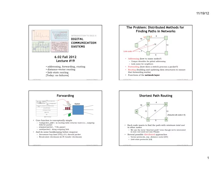
6.02 Fall 2012 Lecture 19, Slide #1
6.02 Fall 2012 Lecture #19
- addressing, forwarding, routing
- distance-vector routing
- link-state routing
[Today: no failures]
6.02 Fall 2012 Lecture 19, Slide #2
The Problem: Distributed Methods for Finding P aths in Networks
L2 4 L0 B D 19 L1 15 A 11 13 Link costs 7 C E 5
- Addressing (how to name nodes?)
– Unique identifier for global addressing – Link name for neighbors
- Forwarding (how does a switch process a packet?)
- Routing (building and updating data structures to ensure
that forwarding works)
- Functions of the network layer
6.02 Fall 2012 Lecture 19, Slide #3
Forwarding
Switch
- Core function is conceptually simple
– lookup(dst_addr) in routing table returns route (i.e., outgoing
link) for packet
– enqueue(packet, link_queue) – send(packet) along outgoing link
- And do some bookkeeping before enqueue
– Decrement hop limit (TTL); if 0, discard packet – Recalculate checksum (in IP, header checksum)
6.02 Fall 2012 Lecture 19, Slide #4
B C D E A 4 11 5 13 15 19 7 (Assume all costs ≥ 0)
Shortest Path Routing
- Each node wants to find the path with minimum total cost
to other nodes
– We use the term “shortest path” even though we’re interested in min cost (and not min #hops)
- Several possible distributed approaches