10-12-2019 Outline Summary of Mondays lesson Monitoring and data - - PDF document

10-12-2019 1

Dan Jensen IPH, KU

Monitoring and data filtering – DLM II

Outline

Summary of Monday’s lesson Examples of when classical methods will suffice, and when they will not

• Break (10 minutes)

Defining variance components for the DLM

• Break

Exercises (incl. Mandatory Report 3)

Summary of Monday’s lesson

Summary of Monday’s lesson

DLM: Dynamic Linear Model

• Two equations: System eq. & observation eq.
• Updated with each new observation using the Kalman filter
• 8 lines of math - Bayesian updating
• The Adaptive coefficient (AC) determines how much the

parameter vector should be adjusted

• The AC serves the same purpose in the DLM as lambda serves

in the EWMA. However, the AC is affected by both the

• bservational variance and the system variance

The DLM can be used for e.g.:

• Alarm systems (remember the ”normality hypothesis”)
• Decision support (look into the future with current knowlegde)
• Effect estimation (strip away the noise - see an effect of the change?)

The forecast errors can be standardized

• If the model is appropriate for the data, the standardized forecast

errors should follow a standard normal distribution (mean = 0, SD = 1)

The Kalman filter

• Updating the DLM (the adaptive coefficient)

Prior information: 1-step forecast information: Adaptation information Filtered (posterior) information Prior mean Prior variance Forecast Forecast variance Adaptive coefficient Forecast error Filtered mean Filtered variance Adaptive coefficient [0;1] Incorporate external information

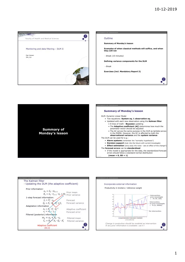
Productivity in broilers / reference weight Change in production should be modeled as intervention If any prior information is available: use it !

Intervention, prior knowlegde Δ ~ N (70, 100) Intervention, no prior knowlegde Δ ~ N (0, 20000) No intervention

10-12-2019 2

Monitoring Deviations from the model

First of all: use standardized errors: Other monioring methods, e.g.: V-mask, Bayesian networks, neural networks, etc.

The model removes auto-correlation

When are the classical methods enough?

Shewart control chart and/or EWMA OK:

• The observations can (reasonably) be assumed to be

mutually independent

• I.e. none or low auto-correlation
• If there is auto-correlation, but no systematic trend is

expcted: EWMA  forecast errors

• Low observation frequency (e.g. quarterly or yearly)
• Remember Thomas’ slide on the ADG of

slaughter pigs!

• High observation level

(e.g. whole herd, not pens or individuals)

• External or prior information is not availible or won’t be

considered Examples:

DLM is needed:

• External and/or prior information should be considered

(Bayesian updating)

• Systematic changes over time are expected
• High observation frequency, e.g. from sensors
• Low-level observations

(individuals or smaller groups of animals) Examples:

10-12-2019 3

Specification of variance components

C0 Prior variance – how uncertain are we of our prior mean? V Observational variance – how uncertain are we of the observed values? W System variance – how uncertain re we in the stability of the system?

Specification of variance components

• Wt using discount factor

Discount factor (δ) as an aid to choosing Wt Discount factor δ can be used if W is unknown - 0 < δ < 1 we know that W is a fixed proportion of C Rt = Ct-1 + W → Rt = Ct-1 / δ For a process in control we use the value of delta that minimize the sum of the squares of the forecast errors et

(like lambda for the EWMA!)

Specification of variance components

• Wt using discount factor

Delta = 0.01 Meaningful range!

Specification of variance components

• Wt using discount factor

Daily gain example High value of delta: small system (evolution) variance W, slow adaptation to new information Low value of delta: very adaptive model This is the opporsite of how lambda works in the EWMA! NB: lower delta can be used for modeling intervention !

10-12-2019 4

Specification of variance components

• Wt using discount factor

Daily gain example For a process in control we use the value of delta that minimize the sum of the squares of the forecast errors et

(like lambda for the EWMA!)

0.59

MA window: here 15 obs. (7 each side)

Specification of variance components

• V based on 2-sided moving average

If you have ”healthy/normal” data availible for learning!

Specification of variance components

• other methods

The expectation maximation (EM) algorithm by Dempster et al. (1977): Assumes that learning ata is availible!

• 1. Start with some inital guess for V and W (and C0)
• 2. Run the DLM om the learning data
• 3. Apply the smoothening to the raw and DLM-filtered data
• 4. Adjust the values of V and W
• 5. (Check the sum of squared errrors (SSE))
• 6. Repeat until convergence or SSE is no longer reduced

Reference analysis, described in detail by West and Harrison (1997): If no learning data is availible!

• 1. Estimate mt, Ct, W and V based on the first few observations
• 2. For more details, see Example 8.7 on page 104 in the Advanced topics

book.