1. Z-transform the step re- sponse to obtain Y s ( z ) . Discrete - PowerPoint PPT Presentation

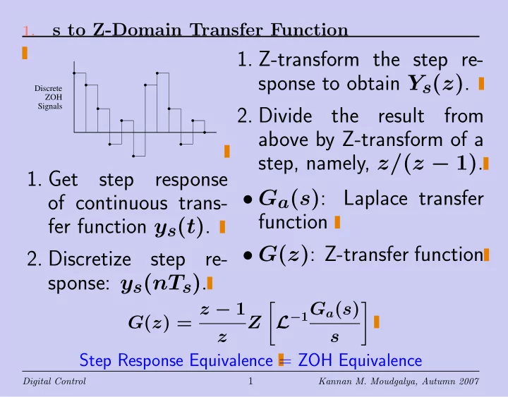
s to Z-Domain Transfer Function 1. 1. Z-transform the step re- sponse to obtain Y s ( z ) . Discrete ZOH Signals 2. Divide the result from above by Z-transform of a step, namely, z/ ( z − 1) . 1. Get step response • G a ( s ) : Laplace transfer of continuous trans- function fer function y s ( t ) . • G ( z ) : Z-transfer function 2. Discretize step re- sponse: y s ( nT s ) . G ( z ) = z − 1 L − 1 G a ( s ) � � Z z s Step Response Equivalence = ZOH Equivalence 1 Digital Control Kannan M. Moudgalya, Autumn 2007

Important Result from Differentiation 2. Recall ∞ z 1( n ) a n ↔ a n z − n , � z − a = n =0 Differentiating w.r.t. a , ∞ z na n − 1 z − n � ( z − a ) 2 = n =0 z na n − 1 1( n ) ↔ ( z − a ) 2 2 z n ( n − 1) a n − 2 1( n ) ↔ ( z − a ) 3 2 Digital Control Kannan M. Moudgalya, Autumn 2007

ZOH Equivalence of 1 /s 3. The step response of Taking Z-transforms 1 /s is 1 /s 2 . In time T s z Y s ( z ) = domain, it is, ( z − 1) 2 y s ( t ) = L − 1 1 s 2 = t Divide by z/ ( z − 1) , to get the ZOH equivalent Sampling it with a pe- discrete domain transfer riod of T s , function y s ( nT s ) = nT s T s G ( z ) = z − 1 3 Digital Control Kannan M. Moudgalya, Autumn 2007

ZOH Equivalence of 1 /s 2 4. The step response of Take Z-transform 1 /s 2 is 1 /s 3 . In time Y s ( z ) = T 2 s z ( z + 1) domain, it is, 2( z − 1) 3 y s ( t ) = L − 1 1 s 3 = 1 2 t 2 . Dividing by z/ ( z − 1) , we get Sampling it with a pe- G ( z ) = T 2 s ( z + 1) riod of T s , 2( z − 1) 2 y s ( nT s ) = 1 2 n 2 T 2 s 4 Digital Control Kannan M. Moudgalya, Autumn 2007

ZOH Equivalent First Order Transfer Function 5. Find the ZOH equivalent of K/ ( τs + 1) . � � Y s ( s ) = 1 K 1 1 τs + 1 = K s − s + 1 s τ � 1 − e − t/τ � y s ( t ) = K , t ≥ 0 � 1 − e − nT s /τ � y s ( nT s ) = K , n ≥ 0 Kz (1 − e − T s /τ ) z z � � Y s ( z ) = K = z − 1 − z − e − T s /τ ( z − 1)( z − e − T s /τ ) Dividing by z/ ( z − 1) , we get G ( z ) = K (1 − e − T s /τ ) z − e − T s /τ 5 Digital Control Kannan M. Moudgalya, Autumn 2007

ZOH Equivalent First Order Transfer Function 6. - Example Sample at T s = 0 . 5 Scilab output is, and find ZOH equivalent 0 . 9546 G ( z ) = trans. function of z − 0 . 9048 10 = 10(1 − e − 0 . 1 ) G a ( s ) = 5 s + 1 z − e − 0 . 1 Scilab Code: In agreement with the Ga = tf(10,[5 1]); formula in the previous G = ss2tf(dscr(Ga,0.5)); slide 6 Digital Control Kannan M. Moudgalya, Autumn 2007

Discrete Integration 7. y ( k ) = blue shaded area u ( n ) + red shaded area u ( k − 1) y ( k ) = y ( k − 1) + red shaded area u ( k ) y ( k ) = y ( k − 1) + T s 2 [ u ( k ) + u ( k − 1)] n Take Z-transform: Y ( z ) = z − 1 Y ( z ) + T s U ( z ) + z − 1 U ( z ) � � 2 Bring all Y to left side: Y ( z ) − z − 1 Y ( z ) = T s U ( z ) + z − 1 U ( z ) � � 2 (1 − z − 1 ) Y ( z ) = T s 2 (1 + z − 1 ) U ( z ) 7 Digital Control Kannan M. Moudgalya, Autumn 2007

Transfer Function for Discrete Integration 8. Recall from previous slide Im ( z ) (1 − z − 1 ) Y ( z ) = T s 2 (1 + z − 1 ) U ( z ) × Re ( z ) 1 + z − 1 Y ( z ) = T s 1 − z − 1 U ( z ) 2 1 s ↔ T s z + 1 = T s z + 1 z − 1 U ( z ) 2 z − 1 2 Integrator has a transfer function, G I ( z ) = T s z + 1 2 z − 1 A low pass filter! 8 Digital Control Kannan M. Moudgalya, Autumn 2007

Derivative Mode 9. • Integral Mode: 1 s ↔ T s z + 1 2 z − 1 • Derivative Mode: s ↔ 2 z − 1 T s z + 1 • High pass filter • Has a pole at z = − 1 . Hence produces in partial fraction expansion, a term of the form z z + 1 ↔ ( − 1) n • Results in wildly oscillating control effort. 9 Digital Control Kannan M. Moudgalya, Autumn 2007

Derivative Mode - Other Approximations 10. Backward difference: y ( k ) = y ( k − 1) + T s u ( k ) (1 − z − 1 ) Y ( z ) = T s U ( z ) 1 z Y ( z ) = T s 1 − z − 1 = T s z − 1 U ( z ) 1 z s ↔ T s z − 1 Forward difference: y ( k ) = y ( k − 1) + T s u ( k − 1) (1 − z − 1 ) Y ( z ) = T s z − 1 U ( z ) z − 1 T s Y ( z ) = T s 1 − z − 1 U ( z ) = z − 1 U ( z ) 1 T s s ↔ z − 1 Both derivative modes are high pass, no oscillations, same gains 10 Digital Control Kannan M. Moudgalya, Autumn 2007

PID Controller 11. Proportional Mode: Most popular control mode. Increase in proportional mode generally results in • Decreased steady state offset and increased oscillations Integral Mode: Used to remove steady state offset. Increase in integral mode generally results in • Zero steady state offset • Increased oscillations Derivative Mode: Mainly used for prediction purposes. Increase in derivative mode generally results in • Decreased oscillations and improved stability • Sensitive to noise The most popular controller in industry. 11 Digital Control Kannan M. Moudgalya, Autumn 2007

PID Controller - Basic Design 12. Let input to controller by E ( z ) and output from it be U ( z ) . If gain is K , τ i is integral time and τ d is derivative time, � t e ( t ) + 1 de ( t ) � � u ( t ) = K e ( t ) dt + τ d τ i dt 0 U ( s ) = K (1 + 1 τ i s + τ d s ) E ( s ) = S c ( s ) △ U ( s ) R c ( s ) E ( s ) If integral mode is present, R c (0) = 0 . Filtered derivative mode: � � 1 + 1 τ d s u ( t ) = K τ i s + e ( t ) 1 + τ d s N N is a large number, of the order of 100. 12 Digital Control Kannan M. Moudgalya, Autumn 2007

Reaction Curve Method - Ziegler Nichols Tun- 13. ing • Applicable only to stable systems • Give a unit step input to a stable system and get 1. the time lag after which the system starts responding ( L ), 2. the steady state gain ( K ) and 3. the time the output takes to reach the steady state, after it starts responding ( τ ) R = K /τ K L τ 13 Digital Control Kannan M. Moudgalya, Autumn 2007

Reaction Curve Method - Ziegler Nichols Tun- 14. ing R = K /τ K L τ • Let the slope of the response be calculated as R = K τ . Then the PID settings are given below: K p τ i τ d P 1/RL PI 0.9/RL 3L PID 1.2/RL 2L 0.5L Consistent units should be used 14 Digital Control Kannan M. Moudgalya, Autumn 2007

Stability Method - Ziegler Nichols Tuning 15. Another way of finding the PID tuning parameters is as follows. • Close the loop with a proportional controller • Gain of controller is increased until the closed loop system becomes unstable • At the verge of instability, note down the gain of the controller ( K u ) and the period of oscillation ( P u ) • PID settings are given below: K p τ i τ d P 0 . 5 K u PI 0 . 45 K u P u / 1 . 2 PID 0 . 6 K u P u / 2 P u / 8 Consistent units should be used 15 Digital Control Kannan M. Moudgalya, Autumn 2007

Design Procedure 16. A common procedure to design discrete PID controller: • Tune continuous PID controller by any popular technique • Get continuous PID settings • Discretize using the method discussed now or the ZOH equiv- alent method discussed earlier • Direct digital design techniques 16 Digital Control Kannan M. Moudgalya, Autumn 2007

2-DOF Controller 17. y r T c u G = B R c A − S c R c u = T c r − S c y R c R c It is easy to arrive at the following relation between r and y . y = T c B/A BT c r = r R c 1 + BS c /AR c AR c + BS c Error e , given by r − y is given by BT c r = AR c + BS c − BT c � � e = 1 − r AR c + BS c AR c + BS c 17 Digital Control Kannan M. Moudgalya, Autumn 2007

Offset-Free Tracking of Steps with Integral 18. E ( z ) = A ( z ) R c ( z ) + B ( z ) S c ( z ) − B ( z ) T c ( z ) R ( z ) A ( z ) R c ( z ) + B ( z ) S c ( z ) z − 1 A ( z ) R c ( z ) + B ( z ) S c ( z ) − B ( z ) T c ( z ) z n →∞ e ( n ) = lim lim z A ( z ) R c ( z ) + B ( z ) S c ( z ) z − 1 z → 1 Because the controller has an integral action, R c (1) = 0 : e ( ∞ ) = S c ( z ) − T c ( z ) � = S c (1) − T c (1) � � S c ( z ) S c (1) � z =1 This condition can be satisfied if one of the following is met: T c = S c T c = S c (1) T c (1) = S c (1) 18 Digital Control Kannan M. Moudgalya, Autumn 2007