1. The code that we have written is, as I pointed out already, a - - PowerPoint PPT Presentation

DNS of Multiphase Flows — Simple Front Tracking

Direct Numerical Simulations of Multiphase Flows-7
 


Results and Tests

Gretar Tryggvason

• 1. The code that we have written is, as I pointed out already, a complete code that can be used to solve

real problems---or as real as the assumption of a two-dimensional flow allows for. Before a numerical code can be used to solve problems it is, however, necessary to gain some familiarity with how it works and how accurate the solution can be expected to be.

DNS of Multiphase Flows — Simple Front Tracking In this lecture we apply our code to a few problems and examine its performance. We will, specifically, look at

• A falling drop and its collision with a no-slip wall
• A rising bubble and its interaction with a no-slip

wall

• The Rayleigh-Taylor instability in a domain with

full slip vertical walls

• 2. Here we test the code on three problems. First we examine a falling drop, similar to the problem

used to test the code, except with a larger density difference. We then examine a rising bubble, which can be set up by simply switching the material parameters, and then we simulate the Rayleigh-Taylor instability where a heavy fluid falls into a lighter one. The last one requires minor changes in the code to account for the different interface shape.

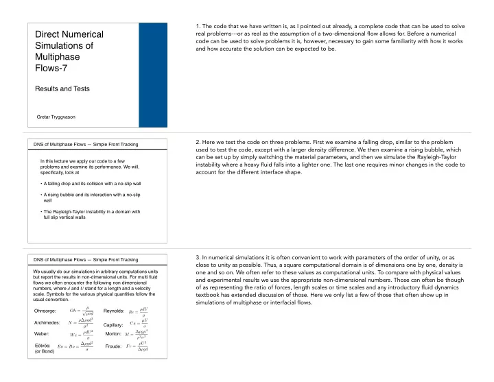
DNS of Multiphase Flows — Simple Front Tracking We usually do our simulations in arbitrary computations units but report the results in non-dimensional units. For multi fluid flows we often encounter the following non dimensional numbers, where d and U stand for a length and a velocity

• scale. Symbols for the various physical quantities follow the

usual convention. Reynolds: Ohnsorge: Weber: Morton: Archimedes: Froude: Eötvös: (or Bond) Capillary: Oh = µ pρσd N = ρ∆ρgd3 µ2 We = ρdU 2 σ Eo = Bo = ∆ρgd2 σ

Re = ρdU µ Ca = µU σ M = ∆ρgµ4 ρ2σ3 Fr = ρU 2 ∆ρgd

• 3. In numerical simulations it is often convenient to work with parameters of the order of unity, or as

close to unity as possible. Thus, a square computational domain is of dimensions one by one, density is

• ne and so on. We often refer to these values as computational units. To compare with physical values

and experimental results we use the appropriate non-dimensional numbers. Those can often be though

• f as representing the ratio of forces, length scales or time scales and any introductory fluid dynamics

textbook has extended discussion of those. Here we only list a few of those that often show up in simulations of multiphase or interfacial flows.

DNS of Multiphase Flows

A Falling Drop Hitting a Wall

• 4. We start with the falling drop. We have already presented results for a falling drop using a 32 by 32
• grid. Here we will look at that problem again, but to make it slightly more interesting we increase the

ratio of the density of the drop to the ambient fluid by ten. Although many multiphase flows are found in high-pressure environments where the density of air is much higher than atmospheric density, many experimental studies are done under atmospheric conditions. Thus, high-density ratios are often of relevance.

DNS of Multiphase Flows — Simple Front Tracking

For a falling drop, as well as a rising bubble, the velocity can be written as a function of the various parameters specifying the problem, as well as time Notice that we include gravity multiplied by the density difference, sine that is the effective buoyancy force. Using the diameter d, drop density, and density difference times gravity, as the repeated variables we find that the non-dimensional relationship is: Or where

U = f(ρd, µd, ∆ρg, σ, d, ρo, µo, t) ρU 2 ∆ρgd = f ρ∆ρgd3 µ2 , ∆ρgd2 σ , ρd ρo , µd µo , s t2∆ρg ρd ! Fr = f(N, Eo, r, m, τ) Fr = ρU 2 ∆ρgd, N = ρ∆ρgd3 µ2 , Eo = ∆ρgd2 σ , r = ρd ρo , m = µd µo , τ = s t2∆ρg ρd

• 5. For the falling drop the diameter of the drop, its density, and gravity, surface tension and viscosity, as

well as the density and viscosity of the ambient fluid, completely specify the problem. Sometimes the density and viscosity of the ambient fluid play smaller roles, particularly if the drop falls only a short

• distance. Generally, the evolution also depends on time. Notice that we include gravity multiplied by

the density difference, since that is the effective buoyancy force. Taking the drop diameter, the drop density, and gravity multiplied by the density difference, as the repeated variables we find that the problem is governed by two non-dimensional numbers, the ratios of the densities and the viscosities, and time. The results, also made non-dimensional by the repeated variables, are therefore a function of these numbers. Thus, the velocity of the drop, represented by the Froude number, or velocity divided by the density difference, gravity and the drop diameter, is a function of the Eotvos and the Archimedes numbers, the density and viscosity ratios and for unsteady problems it is also a function of the appropriately non-dimensional time.

DNS of Multiphase Flows — Simple Front Tracking

We can select other repeated variables to obtain other relationships, but in all cases the problem is specified by two non-dimensional numbers, plus the ratio of the densities and viscosities. The particular non-dimensional numbers selected usually depend on the various limiting cases we want to explore. Sometimes we can ignore the dependency on the viscosity

• r surface tension, in which case the dynamics depends
• nly on one non-dimensional number. If both can be

ignored the problem is even simpler and is described by

• ne non dimensional number being equal to a constant.
• 6. Before moving on we note that the importance of non-dimensional numbers goes far beyond just

allowing us to run our simulations in any units we fancy. Often they can help us to identify limiting cases where we can ignore certain effects, thus simplifying our studies. For drops, it is often found that the effects of viscosity are small, once the Archimedes number is high enough, at least for short enough

• time. Thus, we would expect that once our N is high enough so that the results have stopped changing,

we do not need to increase it further. Since computing very low viscosity can be difficult, or at least time consuming, this simplifies our studies. Similar observations can be made about surface tension, particularly once it is high enough.

DNS of Multiphase Flows — Simple Front Tracking

%=============================================================== Lx=1.0; Ly=1.0; gx=0.0; gy=-100.0; sigma=10; % Domain size and rho1=0.1; rho2=2.0; m1=0.01; m2=0.2; % physical variables unorth=0; usouth=0; veast=0; vwest=0; time=0.0; rad=0.15; xc=0.5; yc=0.7; % Initial drop size and location %-------------------- Numerical variables ---------------------- nx=32; ny=32; dt=0.001; nstep=200; maxit=200; maxError=0.001; beta=1.5; Nf=100;

This gives the following non-dimensional numbers: Galileo Number Eörtvös Number

This is the problem that we have been using to test our code, except here we will take the density and viscosity ratios to be larger. The physical and numerical parameters are specified in the first few lines of the code Eo = ∆ρgd2 σ = 1.9 ⇥ 100 ⇥ 0.32 10 = 1.71

N = ρ∆ρgd3 µ2 = 2 ⇥ 1.9 ⇥ 1 ⇥ 100 ⇥ 0.33 0.22 = 256.5 r = ρd ρo = 2.0 0.1 = 20 m = µd µo = 0.2 0.01 = 20

Property ratios

• 7. Except for the density and viscosity of the ambient gas, we use the parameters used already. Those

are specified at the beginning of the code. Thus Lx and Ly are one, gx is zero but gy is negative 100, the density of the ambient fluid is 0.1 and the drop density is 2. Similarly, the viscosity of the ambient fluid is 0.01 and the drop viscosity is 0.2. Surface tension is 10. The tangent velocities on all four boundaries are zero. The drop radius is 0.15 and it is initially located at x = 0.5 and y = 0.7. We start by using a grid with 32 by 32 pressure control volumes and a time step of 0.001. We will follow the solution for 200 time steps, or up to time 0.2. For the pressure equation we specify an error of 0.001, but we also set the maximum number of iterations to 200.

DNS of Multiphase Flows Simulation of a drop that falls

• nto a rigid wall

and bounces slightly N=256.5 Eo=1.71 ρb/ρl=20 µb/µl=20 A 32 by 32 grid.

• 8. For a 32 by 32 grid the code runs fast enough so that it can be run interactively and the drop
• bserved as it falls. The evolution is very similar to what we saw earlier for the lower density ratio. The

drop deforms slightly as it falls, flattens as it collides with the wall, rebounds slightly and then settles on the wall.

DNS of Multiphase Flows For initial checks of the code, we can use relatively benign parameters, where we do not expect numerical difficulties and the resolution required for convergence is modest. Then we ask: Does it look right? Is the solution as symmetric as it should be? Does rotating or flip the problem give the same solution? Can we test some aspects of the code using analytical solutions? Does the solution converge under grid refinement?

9-1. If we do everything correctly, we expect the numerical solution to be an approximation to an exact solution of the governing equations. At this point, however, we do not know how accurate our solution is or, for that matter, if it is correct. Assuming that our code runs, there are two main reasons that the answer may not be correct. The first is programming errors and the second is numerical errors. Our goal is to eliminate the first and understand the second. For the first part it is convenient to work with “benign” parameters, such as a small density ratio and modest values of viscosity and surface tension, where we are reasonably certain that we will not run into any numerical difficulties. If we have an analytical solution then we can, of course, compare the results with it. In most cases an analytical solution is, however, only available for simple special situations, such as a spherical drop in Stokes flow, that only tests part of the code. In many cases we can use a technique called the method of manufactured solutions, and although it is a great way to check codes, it is a bit of an over kill here. Thus, we are limited to a relatively modest number of things to check.

DNS of Multiphase Flows For initial checks of the code, we can use relatively benign parameters, where we do not expect numerical difficulties and the resolution required for convergence is modest. Then we ask: Does it look right? Is the solution as symmetric as it should be? Does rotating or flip the problem give the same solution? Can we test some aspects of the code using analytical solutions? Does the solution converge under grid refinement?

9-2. First of all, does the solution look correct? If it does not, the probability of an error is far higher than that we have discovered an unexpected behavior. Secondly, is the solution as symmetric as we expect it to be? What about if we let gravity point in the opposite direction? Or to the left or right? Does the solution still look the same? Finally, does the solution converge under grid refinement, where we change both the spatial and the temporal resolution? If we are using benign parameters, it should converge quickly. For the codes that we have presented so far we have done each of those tests for the falling droplet.

DNS of Multiphase Flows Looking at how the velocity and the marker function evolve in time is usually the first step in examining the results. In many cases, however, we desire a more quantitative description of the evolution. This is useful for

• Assessing the convergence of the solution as the numerical

parameters, such as the grid resolution, are varied

• Quantifying how the solution changes as the physical

parameters describing the problem are changed The diagnostic variables, or the quantities of interest, can be defined in several ways, but here we focus only on the simplest

• nes, such as the area of the drop and the location and

velocity of its centroid

• 10. While checking the code for errors is usually a one-time task, examining the convergence must be

done for every new problem that we simulate. Before doing that for the falling drop problem, we need to decide how we evaluate convergence. Looking at the velocity and the marker function and how they evolve in time is certainly the first step, but usually we desire a more quantitative description of the

• evolution. Such description is not only useful to assess the convergence as the numerical parameters,

such as the grid resolution are varied, but also to describe how the solution changes as the physical parameters are changed. The diagnostic variables, or the quantities of interest, can be defined in several ways, but for our purpose we focus only on the simplest ones, such as the area of the drop and the location and velocity of its centroid.

DNS of Multiphase Flows The area of the drop should be constant since the flow is incompressible, and monitoring the area serves as a check

• n the accuracy of the computations.

To compute the area as well s several other quantities of interest it is often useful to convert the elementary definition as a volume or area integral to a surface integral since surface integrals can be found with a high degree of

• accuracy. Thus, the area is given by:

A = Z da = Z 1da = 1 2 Z ⇣∂x ∂x + ∂y ∂y ⌘ da = 1 2 Z r · x = 1 2 I x · nds

Area of drop

• 11. For our problem we know that the volume, or area in our case, should be conserved since the flow

is incompressible. We also expect the centroid of the drop in the horizontal direction to remain

• unchanged. Thus, these are two obvious quantities to monitor. The centroid in the vertical direction

does, obviously, change but it also is an obvious quantity to monitor, as is the centroid velocity. Thus, here we will examine how the drop area and the location and velocity of the centroids evolve with time. These quantities can be computed in different ways, but here we integrate over the interface. The droplet volume is defined as the volume integral of the interior of the drop. In two-dimensions this is an area integral and to convert it into an integral over the surface of the drop we first note that unity can be written as half the divergence of the position vector. That is, the x derivative of x plus the y derivative of y is two. Using the divergence theorem the volume integral can now be written as a surface integral. Notice that we could have used either the x derivative of the horizontal component or the y derivative of the vertical component, but using the average avoids biasing the results in either direction.

DNS of Multiphase Flows

R XC = 1 A Z xda = 1 A Z (x, y)da = 1 2A Z ⇣∂x2 ∂x , ∂y2 ∂y ⌘ da = 1 2A Z r ⇣ x2 + y2⌘ da = 1 2 I ⇣ x2 + y2⌘ nds Z VC = dXC dt

The velocity of the drop centroid can be found by differencing the location of the centroid Centroid of drop The velocity of the drop centroid can also be found by by integrating over the boundary, but this is usually less accurate. Other elementary quantities of interest include the interface length which is found by S = I ds

• 12. The centroid of the drop is defined as the volume integral of the position vector divided by the

volume, and the volume integral can be rewritten as a surface integral by recognizing that the position vector is half the divergence of a vector whose components are the coordinates squared. The centroid velocity, defined as the average velocity of the drop, can be computed by simply taking the time derivative of the centroid location. It can also be found as a surface integral, but generally we find that to be less accurate, particularly for low resolutions. The total interface length (or surface area in three- dimension) is also an important quantity of interest, since it is directly related to the surface energy. This can be found in a straightforward way.

DNS of Multiphase Flows

%================= DIAGNOSTICS ============================= Area(is)=0; CentroidX(is)=0; CentroidY(is)=0; Time(is)=time; for j=1:Nf, Area(is)=Area(is)+... 0.25*((xf(j+1)+xf(j))*(yf(j+1)-yf(j))-(yf(j+1)+yf(j))*(xf(j+1)-xf(j))); CentroidX(is)=CentroidX(is)+... 0.125*((xf(j+1)+xf(j))^2+(yf(j+1)+yf(j))^2)*(yf(j+1)-yf(j)); CentroidY(is)=CentroidY(is)-... 0.125*((xf(j+1)+xf(j))^2+(yf(j+1)+yf(j))^2)*(xf(j+1)-xf(j)); end CentroidX(is)=CentroidX(is)/Area(is);CentroidY(is)=CentroidY(is)/Area(is); % plot(Time,Area,'r','linewidth',2); axis([0 dt*nstep 0 0.1]); % set(gca,'Fontsize',18, 'LineWidth',2) % T1=Time;A1=Area;CX1=CentroidX;CY1=CentroidY; % T2=Time;A2=Area;CX2=CentroidX;CY2=CentroidY;

Here we use integration over the front to compute the area and the centroids. The code to do so is:

• 13. In the current code we collect the various diagnostics as the code runs so we need to add a few

lines to do that at the end of the time loop. We also have included a few commands to plot these quantities, as well as to save them under a different name. This is useful when we are doing grid refinement or parameter studies and want to rerun the code several times and compare the results.

DNS of Multiphase Flows

0.05 0.1 0.15 0.2 0.06 0.062 0.064 0.066 0.068 0.07 0.072 0.074 0.076 0.078 0.08 0.05 0.1 0.15 0.2

• 10
• 8
• 6
• 4
• 2

2 4 0.05 0.1 0.15 0.2 0.1 0.2 0.3 0.4 0.5 0.6 0.7

0.1 0.2 0.3 0.4 0.5 0.6 0.7 0.8 0.9 1 0.1 0.2 0.3 0.4 0.5 0.6 0.7 0.8 0.9 1 0.1 0.2 0.3 0.4 0.5 0.6 0.7 0.8 0.9 1 0.1 0.2 0.3 0.4 0.5 0.6 0.7 0.8 0.9 1 0.1 0.2 0.3 0.4 0.5 0.6 0.7 0.8 0.9 1 0.1 0.2 0.3 0.4 0.5 0.6 0.7 0.8 0.9 1

128 by 128 32 by 32 64 by 64 The front, the velocity field, and the marker function at time 0.2 Drop area versus time Y-centroid versus time Y-velocity versus time Results for three grids

• 14. The top three frames show the front, the velocity field and the marker function for three different

resolutions, 32 by 32, 64 by 64, and 128 by 128 grids, at time 0.2, when the drop has collided with the wall and rebounded slightly. Although the droplet shape is similar in all three frames, it is also obvious that there are slight differences, particularly between the first two frames. The three plots at the bottom show the area of the drop, the distance of the drop centroid from the bottom wall and the centroid velocity, versus time, for all three runs. The black line is for the lowest resolution and the red line is for the finest one. On the coarsest grid the drop looses a little bit of mass, particularly when it first collides with the wall, but overall the results agree well, particularly for the two finest grids.

DNS of Multiphase Flows

A Rising Bubble Colliding with a Wall

• 15. Our code is, at least in principle, capable of solving a wide range of problems involving two

immiscible fluids. It is, however, not written as a multipurpose code, so in most cases we need to change the code to do a new problem. The simplest change is to examine bubbles, or light drops, instead of heavy drops. To do so we only need to change the material properties so that buoyancy drives the bubble upwards, instead of down.

DNS of Multiphase Flows A bubble is the inverse of a drop, where a light fluid blob moves in a heavy liquid. We will make the domain twice as long, so that the bubble will have time to reach an approximate steady state before hitting the top wall

Galileo Number Eörtvös Number

N = ρ∆ρgd3 µ2 = 2 × 1.95 × 100 × 0.33 0.12 = 1.053 × 103 Eo = ∆ρgd2 σ = 1.95 × 100 × 0.32 10 = 1.755 Lx=1.0;Ly=2.0;gx=0.0;gy=-100.0; sigma=10; % Domain size and rho1=2.0; rho2=0.05; m1=0.1; m2=0.005; % physical variables unorth=0;usouth=0;veast=0;vwest=0;time=0.0; rad=0.15;xc=0.5;yc=0.3; % Initial bubble size and location %-------------------- Numerical variables ---------------------- nx=32;ny=64;dt=0.00125;nstep=400; Nf=100; maxit=200;maxError=0.001;beta=1.5;

• 16. We change the top of the file to modify the material parameters. The density of the ambient fluid is

2 and the bubble density is 0.05. Similarly, the viscosity of the ambient fluid is 0.1 and the bubble viscosity is 0.005. Surface tension is 10 and gravity is -100, as for the simulation of the drop. In addition, we make the computational domain taller so that the bubble can rise for a longer distance. The tangent velocities on all four boundaries are zero. The bubble radius is 0.15 and it is initially located at x = 0.5 and y = 0.3. We start by using a grid with 32 by 64 pressure control volumes and a time step of 0.00125. We will follow the solution for 400 time steps, or up to time 0.5. For the pressure equation we specify an error of 0.001, and set the maximum number of iterations to 200, as before.

DNS of Multiphase Flows

0.2 0.4 0.6 0.8 1 0.2 0.4 0.6 0.8 1 1.2 1.4 1.6 1.8 2

TODO

Simulation of a bubble rising in a narrow domain and colliding with the top rigid wall N=1.053 x 103 Eo=1.755 ρb/ρl=40 µb/µl=20 A 32 by 64 grid.

• 17. The bubble moves upward due to buoyancy, staying more or less spherical, quickly reaching a

steady state velocity and leaving a significant wake. As it reaches the top it flattens slightly.

DNS of Multiphase Flows The front, the velocity field, and the marker function

• n three different grids at time 0.5

0.1 0.2 0.3 0.4 0.5 0.01 0.02 0.03 0.04 0.05 0.06 0.07 0.08 0.09 0.1 0.1 0.2 0.3 0.4 0.5 0.2 0.4 0.6 0.8 1 1.2 1.4 1.6 1.8 2 0.1 0.2 0.3 0.4 0.5

• 0.5

0.5 1 1.5 2 2.5 3 3.5 4

Centroid versus time Area versus time Centroid Velocity versus time

Grid 1: nx=32; ny=64; dt=0.00125; nstep=400; Nf=100; Grid 2: nx=2*32; ny=2*64; dt=0.5*0.00125; nstep=2*400; Nf=2*100; Grid 3: nx=4*32; ny=4*64; dt=0.125*0.00125; nstep=8*400; Nf=4*100;

• 18. We again repeat the simulation on three grids and top three frames show the front, the velocity

field and the marker function for three different resolutions, 32 by 64, 64 by 128, and 128 by 256 grids, at time 0.5, when the bubble has collided with the top wall. Although the bubble shape is similar in all three frames, it is also obvious that there are slight differences, particularly between the first two

• frames. The three plots on the bottom show the area of the bubble, the distance of the bubble

centroid from the bottom wall and the centroid velocity, versus time, for all three runs. The black line is for the lowest resolution and the red line is for the finest one. The mass conservation here is obviously not as good as for the drop, where we had to expand the vertical axis to see the difference between the different resolutions. It does, however, improve with increasing resolution and there are only minor differences in the curves for the centroid location and the velocities for the finer two grids.

DNS of Multiphase Flows

The Rayleigh- Taylor Instability

• 19. The mixing of two fluids, as a heavy fluid initially placed above a lighter one, falls down and the

light fluid rises, is a classical problem in computations of multifluid flows. Computationally it is fairly

• simple. We put heavy fluid in the top part of the domain and perturb the interface to initiate the
• motion. Experimentally it is more complex. In some cases the heavy and the light fluids are initially

separated by a membrane, which is removed as quickly as possible, but in other cases the heavy fluid is initially at the bottom of a container that is accelerated downward, using devices ranging from rubber bands to rocket motors.

DNS of Multiphase Flows The Rayleigh-Taylor instability is one of the classical test problems for multiphase simulations. Initially a heavy fluid sits above a lighter one, but once the interface is perturbed slightly the heavy fluid and the light one trade places. For this problem we need to change our code slightly:

• We change the boundary condition on the vertical walls to

full-slip for the flow solver, and

• The front now stretches between the walls instead of being

closed

• The boundary conditions for the front, where it meets the

walls is simplified by assuming that the interface is flat there

• 20. To simulate the evolution of the Rayleigh-Taylor instability we need to make minor changes in the
• code. The interface does, in particular, no longer enclose an isolated blob, but extends from the left to

the right boundary. We will assume that the evolution is symmetric and that the side walls can be taken to be full slip walls. This allows us to assume that the slope of the interface at the side walls is zero which simplifies the implementation of the boundary condition for the front.

DNS of Multiphase Flows Making the vertical walls full-slip is a very minor change. We want the shear stress there to be zero, so the velocity gradient is zero and this is accomplished by putting the tangent velocity at the ghost point equal to the first tangent velocity inside the domain. The changes to the front are also relatively simple. The biggest decision is whether there is a front point on the boundary or whether we let put the boundary between the first point and the second one? Here we choose to do the latter, so that the first and the last points are ghost points outside the computational domains.

• 21. Making the vertical walls full-slip is a very minor change. We want the shear stress there to be zero,

so the velocity gradient is zero and this is accomplished by putting the tangent velocity at the ghost points equal to the first tangent velocity inside the domain. The changes to the front are also relatively

• simple. Instead of forming a closed circle, it now stretches across the domain, from the left to right. We

need to decide exactly how we handle the endpoints and here we use ghost points so the first point is

• utside the domain and the left boundary falls between the first and the second point. The right

boundary is handled in the same way.

DNS of Multiphase Flows The changes in the code are relatively minor. First of all, we modify the physical and numerical parameters slightly and change the initial conditions:

%======================================================== Lx=1.0;Ly=2.0;gx=0.0;gy=-100.0; sigma=5.0; % Domain size and rho1=1.0; rho2=4.0; m1=0.01; m2=0.05; % physical variables unorth=0;usouth=0;veast=0;vwest=0;time=0.0; %-------------------- Numerical variables ---------------------- nx=32; ny=64; dt=0.00125; nstep=300; maxit=200; maxError=0.001; beta=1.5; Nf=100; %-------------------- Initial Conditions ----------------------- r=zeros(nx+2,ny+2)+rho1;m=zeros(nx+2,ny+2)+m1; % Set density and viscosity for i=1:nx+2,for j=1:ny+2; % for the domain and the drop if(y(j)>1.2+0.1*cos(2.0*pi*x(i))), r(i,j)=rho2; m(i,j)=m2; chi(i,j)=1.0; end, end, end

• 22. Changes in the code are minor. First of all, we need to modify the physical and numerical

parameters at the beginning of the code. We take Lx to be one and Ly to be two, as for the bubble

• simulation. gx is zero but gy is negative 100, the density of the heavy fluid at the top is 4 and the

density of the light fluid at the bottom is 1. Similarly, the viscosity of the heavy fluid is 0.05 and the viscosity of the light fluid is 0.01. Surface tension is 5. The tangent velocities on the top and bottom boundaries are zero. We start by using a grid with 32 by 64 pressure control volumes and a time step of 0.00125. We will follow the solution for 300 time steps, or up to time 0.375. For the pressure equation we specify an error of 0.001, but we also set the maximum number of iterations to 200. When we compute the relevant non-dimensional numbers, we will use the properties of the top fluid and take the width of the domain as a length scale. The initial conditions must be modified and we take the interface to run across the domain at y=1.2, perturbing it with a cosine wave of amplitude 0.2. Here we have hardcoded the location and perturbation of the interface but we could, of course, make those variables as we did for the droplet size and location.

DNS of Multiphase Flows Then we need to change a few things

After finding the velocity, we add a line: uf(2)=0; uf(Nf+1)=0; % Make sure the endpoint move along wall After moving the points we change a line xf(1)=-xf(2);yf(1)=yf(2);xf(Nf+2)=2*Lx-xf(Nf+1);yf(Nf+2)=yf(Nf+1); After finding the marker function we add a line: chi(1,:)=chi(2,:); chi(nx+2,:)=chi(nx+1,:); % Correct density on sides Before updating the velocities we modify the boundary conditions v(1,1:ny+1)=v(2,1:ny+1);v(nx+2,1:ny+1)=v(nx+1,1:ny+1); Before finding diagnostics we change a line uf(1)=uf(2);vf(1)=vf(2);uf(Nf+2)=uf(Nf+1);vf(Nf+2)=vf(Nf+1); % Front After adding and deleting points we change the updating of the ghost points xf(1)=-xf(2);yf(1)=yf(2);xf(Nf+2)=2*Lx-xf(Nf+1);yf(Nf+2)=yf(Nf+1); Change the plotting slightly: plot(xf(1:Nf+2),yf(1:Nf+2),'k','linewidth',3);pause(0.01)

• 23. Then we change the code to deal with the new situation. We add a line putting the horizontal

velocities of the first and last front point inside the domain to zero, to ensure that they do not drift

• utside the domain. After finding the velocity of the front points we modify the line setting the value of

the ghost points. On the side walls we add a line to set the density at the ghost points equal to density

• f the next interior point, since the interface moves. This is not strictly needed since these points are

not used, but they will look better when we plot the marker. We change the line where the ghost velocities on the vertical walls are specified to impose full slip walls. Before computing the diagnostics we modify the line setting the ghost velocities for the front. And we modify the line setting the location

• f the front ghost points after we add and delete points. Finally we modify the plotting slightly to plot

the whole front.

DNS of Multiphase Flows Simulation of a Rayleigh-Taylor instability where a heavy fluid falls into a lighter one. Nondimensional numbers based on the properties of the heavy fluid and d=1. N=4.8 x 105 Eo=60 ρt/ρb=4 µt/µb=5 A 32 by 64 grid.

24-1. Here we show the evolution of the Rayleigh-Taylor instability as computed on a 32 by 64 grid. The initial growth of the perturbation is very slow, but then it speeds up. The light fluid rising upward is generally referred to as a bubble and the heavy fluid falling down as a spike. This terminology becomes increasingly precise as the density ratio increases, but here, where the heavy fluid is four times denser than the light fluid the evolution is more symmetric, at least at the early stage. As the spike falls, its nose first becomes flatter as the pressure in the light fluid resists its motion and the rim is then pulled

• ff, by the light fluid rushing into the upward moving bubble. These “arms” develop very quickly and

consists of a drop connected to the rest of the heavy fluid by a thin filament. They are, in particular, much smaller than the bubble or the main part of the downward falling spike. The Rayleigh-Taylor instability exemplifies a major challenge in simulations of multifluid and multiphase flows. While initially everything is well behaved and it is easy to get a fully converged solution, at later time we see the formation of very small-scale features that are much smaller than the scales in the initial conditions.

DNS of Multiphase Flows Simulation of a Rayleigh-Taylor instability where a heavy fluid falls into a lighter one. Nondimensional numbers based on the properties of the heavy fluid and d=1. N=4.8 x 105 Eo=60 ρt/ρb=4 µt/µb=5 A 32 by 64 grid.

24-2. These small scales feature are so small that a grid resolution that was perfectly fine before their formation is now totally insufficient. For the single mode Rayleigh-Taylor instability these are, except for very high viscosities, unavoidable. High surface tension can also suppress them, but if we make the surface tension too high the interface becomes stable and the perturbation oscillates instead of growing.

DNS of Multiphase Flows Convergence

0.2 0.4 0.6 0.8 1 0.2 0.4 0.6 0.8 1 1.2 1.4 1.6 1.8 2 0.2 0.4 0.6 0.8 1 0.2 0.4 0.6 0.8 1 1.2 1.4 1.6 1.8 2 0.2 0.4 0.6 0.8 1 0.2 0.4 0.6 0.8 1 1.2 1.4 1.6 1.8 2

Time 0.375

0.2 0.4 0.6 0.8 1 0.2 0.4 0.6 0.8 1 1.2 1.4 1.6 1.8 2 0.2 0.4 0.6 0.8 1 0.2 0.4 0.6 0.8 1 1.2 1.4 1.6 1.8 2 0.2 0.4 0.6 0.8 1 0.2 0.4 0.6 0.8 1 1.2 1.4 1.6 1.8 2

Time 0.25

0.1 0.2 0.3 0.4 0.2 0.4 0.6 0.8 1 1.2 1.4 1.6 1.8 2 0.1 0.2 0.3 0.4 1 2 3 4 5 6 7 8 9

• Max. Amplitude
• Min. Amplitude

Interface Length versus Time 32 x 64 64 x 128 128 x 256

25-1. To check the convergence we examine the solution at two times on three different grids, using 32 by 64, 64 by 128 and 128 by 256 pressure control volume inside the domain. At the earlier time, in the top row, we see that the three resolutions result in essentially identical solutions. At the later time, however, the differences are larger. The shape of the upward moving bubble is nearly the same, and so is the blunt disk like shape moving down into the light fluid. The shape of the “arms” shed from the rim

• f the heavy disk does, however, change with the resolution. This is a common problem in multiphase

flow simulations. The flow often generates scales that are much smaller than the initial scales, and the small scales quickly become under-resolved. For fine enough grids we do, of course expect convergence since eventually viscosity and/or surface tension sets the smallest scales, but the fact that this can happen at orders of magnitude smaller scales than the initial setup often makes it difficult to produce a fully resolved solution. Although we will not discuss this issue here, it is a major one and one that is currently being actively examined. We can quantify the evolution is several different ways but here we do the simplest thing possible.

DNS of Multiphase Flows Convergence

0.2 0.4 0.6 0.8 1 0.2 0.4 0.6 0.8 1 1.2 1.4 1.6 1.8 2 0.2 0.4 0.6 0.8 1 0.2 0.4 0.6 0.8 1 1.2 1.4 1.6 1.8 2 0.2 0.4 0.6 0.8 1 0.2 0.4 0.6 0.8 1 1.2 1.4 1.6 1.8 2

Time 0.375

0.2 0.4 0.6 0.8 1 0.2 0.4 0.6 0.8 1 1.2 1.4 1.6 1.8 2 0.2 0.4 0.6 0.8 1 0.2 0.4 0.6 0.8 1 1.2 1.4 1.6 1.8 2 0.2 0.4 0.6 0.8 1 0.2 0.4 0.6 0.8 1 1.2 1.4 1.6 1.8 2

Time 0.25

0.1 0.2 0.3 0.4 0.2 0.4 0.6 0.8 1 1.2 1.4 1.6 1.8 2 0.1 0.2 0.3 0.4 1 2 3 4 5 6 7 8 9

• Max. Amplitude
• Min. Amplitude

Interface Length versus Time 32 x 64 64 x 128 128 x 256

25-2. In the top frame on the right we plot the maximum and the minimum of the interface versus time and see that those are essentially identical on all three grids. Below, we plot the total length of the interface versus time, and here we see that while the total lengths on the coarser grids are similar, the finest grid results in a shorter interface, as we expect from the interface shape shown on the left.

DNS of Multiphase Flows The current code can easily be modified for many other problems, such as waves, bubbles and drops coalescing with each other or an interface, and more than one bubble or drop. The current code is written assuming a single continuous interface. For complex problems with many bubbles or drops, where there are several unconnected interfaces, a more general interface data structure is generally preferred.

26.The thorough testing of a numerical code has several purposes. First and foremost we need to convince us, and often others, that the code is correct. Part of this can be done using benign parameters, where the solution should converge easily on a relatively coarse grid. This helps us establish that the method is correctly implemented, even if the method has difficulty with the initial conditions and the parameter values that we really want to simulate. A code that works for some parameter set also provides a path to managing more complex problems. We gradually change the physical parameters and when we run into problems, we change the numerical parameters, such as spatial and temporal resolution and maximum iterations, to see if we can get a solution. Even though a code has been thoroughly tested for one problem, it is usually necessary to repeat some of the tests when we apply it to a new problem, to establish the convergence properties and determine what resolution is necessary.