1 Introduction (1/3) So far Control: compare key figures (k) with - - PDF document

1

Dias 1

Monitoring and data filtering

• I. Classical Methods

Advanced Herd Management Cécile Cornou, IPH

Dias 2

Outline

Framework and Introduction Shewart Control chart

• Basic principles
• Examples: milk yield and daily gain
• Alarms

Moving Average Control Chart EWMA Control Chart

• --- Break & exercises

Monitoring autocorrelation

• Model for autocorrelation
• Use EWMA

Concluding remarks

Dias 3

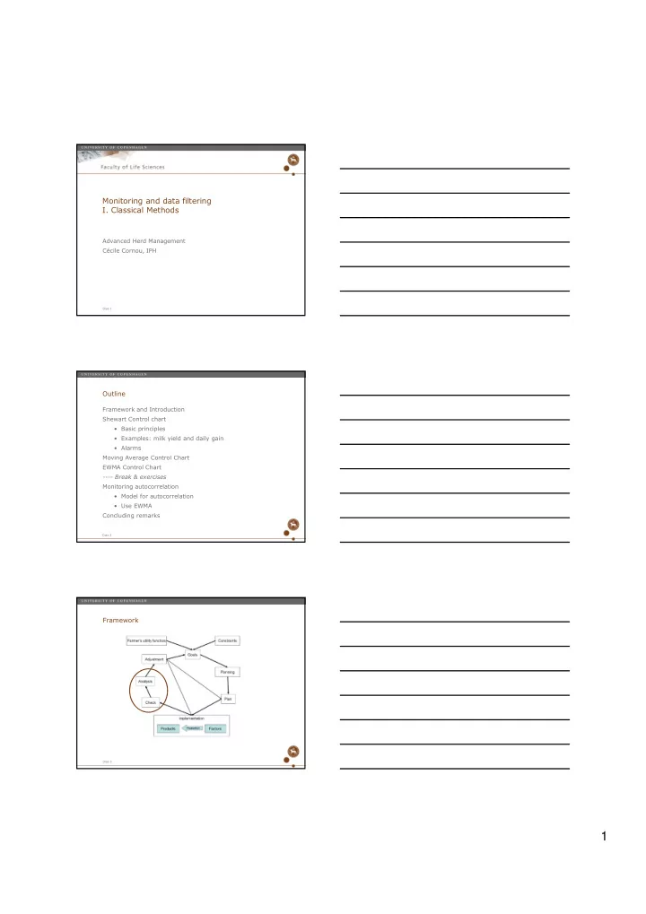
Framework

2

Dias 4

Introduction (1/3)

So far Control: compare key figures (k) with expected results κ = θ + es + eo Deviation: look if significant from a statistical point of view If deviation: adjustement plan or/and implementation Problem: we assume that results can be evaluated without considering results from the previous period

Dias 5

Results from 2 herds 780 790 800 810 820 830 840 850 860 870 880 2 4 6 8 10 12 Quarter Gain (g) Expected Herd A Herd B

Is the conclusion the same in both herds? Introduction (2/3)

Dias 6

Key figures regarded as a time series of observations, treated as a whole How to model the results? κt = θ + est + eot κt : observed value of the key figure θ : true underlying value est : sample error (biological variation) eot : observation error (observation method)

Introduction (3/3)

= θ + νt

3

Dias 7

The Shewart Control Chart: basic principles (1/2)

Upper Control Limit (UCL) Center Line Lower Control Limit (LCL)

Sample number, or time Sample quality characteristic Here: all the points fall inside the CL. Process in control

κ1, κ2, ... κn θ'

Dias 8

Center line = target value

• CL = θ’

Determination of the control limits

• UCLt = θ’ + a σt
• LCLt = θ’ - a σt

Usually distance parameter a = 2 or 3

• If a = 2 : ”2-sigma” control limit

We test the hypothesis H0: θ’ = θ

• a = 2 corresponds to approx. 5% precision level

The Shewart Control Chart: basic principles (2/2)

Dias 9

Target value: CL = θ’ = 25.60 kg for first lactation Control limits: UCLt = θ’ + a σ t LCLt = θ’ - a σ t Standard deviation calculated according to number of cows behind the average

Example 1: milk yield

4

Dias 10

Example 1: milk yield

Shewart control chart, 2-sigma CL

Dias 11

Example 1: milk yield

Shewart control chart, 2-sigma CL

Dias 12

Control and warning limits (1/3)

UCL and LCL determined by a (a=2 <-> p=0.05) Possible that a change in θ is not detected (type II error) Lower a reduces type II but increases type I Possible that alarm is given even though no change (type I error) Choice of significance level / distance parameter: tradeoff between number of type I and II errors. High a reduces type I but increases type II (and vice versa)

5

Dias 13

Control and warning limits (2/3)

Sampling Frequency The more frequent κ is calculated, the higher a Average Run Length ARL=1/q ARL: expected number of obs between 2 out-of-control alarms q is the probability of an arbitrary point exceeding the control limits Average Time to Signal ATS=ARL/ν Sampling frequency defined as ν observations per time unit

Example: Process in control ARL0=1/q=1/p=1/0.05=20 Quaterly obs ATS0=ARL0/ν=20/4=5 Two obs per second ATS0=ARL0/ν=20/2=10

Dias 14

Control and warning limits (3/3)

What is the cost of a type II error? (change not detected)

• Not detected decrease in average milk
• Not detected illness, oestrus

What is the cost of type I error? (false alarm)

• Time spent checking a false alarm
• Risk decrease the reactivity of the farmer to an alarm

Alternative: use of warning limits (fig. 1.5 vs. 2)

Dias 15

Pattern detection

What do we detect?

• Level change, outliers, increase in variation (control limits)
• Trend (increase, decrease), cyclic pattern, autocorrelation

Rules of thumb: 1- One point outside the control limits 2- Two out of three consecutive points outside the warning limits 3- Four out of five consecutive points at a distance of more than σ from the expected level 4- Eight consecutive points on the same side of the expected level

6

Dias 16

Illustration pattern detection

From Example 1

! Rule 4

Dias 17

Precision estimates (σ) Random sampling: 20.2 g Target value: θ’ = CL = 775 g Control limits: UCL = 775 + aσ, a = 2 LCL = 775 − aσ, a = 2

Example 2: daily gain

Dias 18

Example 2: daily gain

Shewart control chart, 2-sigma CL

7

Dias 19

Process out of control 7 obs out of 16 Seasonnal variation is to be expected in slaughter pig production If there is an expected pattern: use of other monitoring techniques to take it into account e.g. other classical techniques (presented next) or state space models (chapter 8) If no expected pattern: further analysis / intervention

Example 2: daily gain

Dias 20

Moving Average Control Charts (1/2)

The moving average is the average of the most recent n observations

, ) (

1 1

n n M

t t n t t

κ κ κ + + + =

− + −

…

n t ≥

with variance

n

2

σ

The moving average control chart is built the same way as the Shewart control chart

Dias 21

Moving Average Control Charts (2/2)

What can we conclude? Using n=4, a=3

8

Dias 22

Exponentially Weighted Moving Average control charts (1/3)

The EWMA is a weighted average of all observations until now 1

) 1 (

−

− + =

t t t

z z λ λκ

with variance, for large t,

      − ≈ λ λ σ σ 2

2 2

t

z

The EWMA control chart is built the same way as the Shewart control chart The most recent observations are given highest weights

Dias 23

Exponentially Weighted Moving Average control charts (2/3)

First lactation, a=2, λ=0.68

Dias 24

Exponentially Weighted Moving Average control charts (3/3)

Choice of lambda:

Small values favor detection of small shifts of θ ! Can take time to detect : small lambda = low weight to new obs

Shewart control chart is suggested for detecting large shifts Combination of EWMA + Shewart for both small and large shifts

9

Dias 25

Monitoring autocorrelated data

Our time series is modeled as κt = θ + νt Assumption: error terms independent Sample error: often autocorrelated due to repeated measurements on same animal, environmental effects... Observation error: often independent but depends of measurement method = θ + est + eot

Dias 26

Daily gain example

Dias 27

Cor r el ati on 650 700 750 800 850 900 650 700 750 800 850 900 P r e v i o s

Daily gain example - Check for autocorrelation

Present versus previous observation Not obvious

Cor r el ati on 650 700 750 800 850 900 650 700 750 800 850 900 P r e v i o s

Present versus same quarter last year Seems clear

10

Dias 28

Milk Yield example - Check for autocorrelation

Present versus previous observation Positive autocorrelation Sample autocorrelation First lactation

Dias 29

A model for autocorrelation

When a model is defined, it is used for prediction of the next

• bservation, given the information available at time t.

t t t t

∈ + =

−1

υ β υ

At time t+1, the true value is observed and the forecast error calculated. where βt is the autoregresive coefficient and Єt is an independent random term First order autoregressive model

) ' ( ' ) ( ˆ

1 1

θ κ β θ κ − + =

+ + t t t

t ) ( ˆ

1 1 1

t e

t t t + + +

− = κ κ

Model Predict next obs. Errors = Observed - predict t t

e υ =

t

e e e ,..., ,

2 1

Dias 30

Control chart – correlated data

Construct a model describing the correlation Use the model to predict next observation Calculate the forecast error = difference between the observed and predicted value Calculate the standard deviation of the forecast error Create a usual control chart for the prediction error

11

Dias 31

EWMA for autocorrelated data

Use EWMA as one-step-ahead predictor for autocorrelated data t t

z ≈

+1

ˆ κ

1 −

− =

t t t

z e κ

Choose λ by minimizing the sum of the squares of the forecast errors

∑

= t i i

e

1 2 The variance of the forecast errors is calculated as

t e

t i i e

∑ =

=

1 2 2

σ

Dias 32

EWMA for autocorrelated data

First order autoregressive model EWMA as predictor

Very similar control charts 2 alarms (EWMA) vs. 1 alarm (autoregr. model) Here autoregr. model performs best EWMA advantage: monitor for level changes without considering the target

Dias 33

Concluding remarks

We have shifted focus from observing a key figure κ at time t to an entire time series (κ1, κ 2,... κ t) We tried to detect changes in process (alarms)

• Raw data (Shewart control chart)
• Averaged data (Moving / Exponentially Moving Average)

We observed autocorrelation: model, EWMA We observed seasonality In the next lecture we will see how to model it using cyclic components