1
play

1 Aspects of Search Quality System Aspects of Evaluation - PDF document

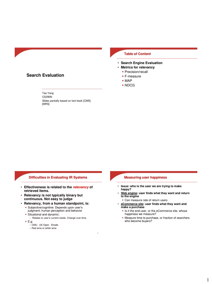
Table of Content Search Engine Evaluation Metrics for relevancy Precision/recall Search Evaluation F-measure MAP NDCG Tao Yang CS290N Slides partially based on text book [CMS] [MRS] Difficulties in Evaluating IR Systems


  1. Table of Content • Search Engine Evaluation • Metrics for relevancy  Precision/recall Search Evaluation  F-measure  MAP  NDCG Tao Yang CS290N Slides partially based on text book [CMS] [MRS] Difficulties in Evaluating IR Systems Measuring user happiness • Issue: who is the user we are trying to make • Effectiveness is related to the relevancy of happy? retrieved items. • Web engine: user finds what they want and return • Relevancy is not typically binary but to the engine continuous. Not easy to judge  Can measure rate of return users • Relevancy, from a human standpoint, is: • eCommerce site: user finds what they want and  Subjective/cognitive: Depends upon user’s make a purchase  Is it the end-user, or the eCommerce site, whose judgment, human perception and behavior  Situational and dynamic: happiness we measure?  Measure time to purchase, or fraction of searchers – Relates to user’s current needs. Change over time.  E.g. who become buyers? – CMU. US Open. Etrade. – Red wine or white wine 3 1
  2. Aspects of Search Quality System Aspects of Evaluation • • Relevancy Response time:  Time interval between receipt of a user query and the • Freshness& coverage presentation of system responses.  Average response time  Latency from creation of a document to time – at different traffic levels (queries/second) in the online index. (Speed of discovery and – When # of machines changes – When the size of database changes indexing) – When there is a failure of machines •  Size of database in covering data coverage Throughputs  Maximum number of queries/second that can be handled • User effort and result presentation – without dropping user queries  Work required from the user in formulating – Or meet Service Level Agreement (SLA)  For example, 99% of queries need to be completed queries, conducting the search within a second.  Expressiveness of query language  How does it vary when the size of database changes  Influence of search output format on the user’s ability to utilize the retrieved materials. System Aspects of Evaluation Relevance benchmarks • Relevant measurement requires 3 elements: • Others 1. A benchmark document collection  Time from crawling to online serving. 2. A benchmark suite of queries  Percentage of results served from cache 3. Editorial assessment of query-doc pairs  Stability: number of abnormal response – Relevant vs. non-relevant spikes per day or per week. – Multi-level: Perfect, excellent, good, fair, poor, bad  Fault tolerance: number of failures that can Precision Retrieved and recall Document Algorithm result be handled. under test Evaluation collection  Cost: number of machines needed to handle Standard Standard queries result – different traffic levels • – host a DB with different sizes Public benchmarks  Smart collection: ftp://ftp.cs.cornell.edu/pub/smart  TREC: http://trec.nist.gov/  Microsoft/Yahoo published learning benchmarks 2

  3. Unranked retrieval evaluation: Precision and Recall Precision and Recall • Precision: fraction of retrieved docs that are irrelevant retrieved Not retrieved relevant = P(relevant|retrieved) & Retrieved Entire & irrelevant • Recall: fraction of relevant docs that are retrieved = documents irrelevant Relevant document documents P(retrieved|relevant) collection relevant retrieved not retrieved & relevant but relevant Relevant Not retrieved not retrieved Relevant Retrieved tp fp Number of relevant documents retrieved recall  Not fn tn Total number of relevant documents Retrieved • Precision P = tp/(tp + fp) Number of relevant documents retrieved precision  • Recall R = tp/(tp + fn) Total number of documents retrieved 10 Determining Recall is Difficult Trade-off between Recall and Precision • Total number of relevant items is sometimes not Returns relevant documents but available: misses many useful ones too The ideal  Use queries that only identify few rare documents 1 known to be relevant Precision 0 1 Recall Returns most relevant documents but includes lots of junk 11 12 3

  4. F-Measure E Measure (parameterized F Measure) • A variant of F measure that allows weighting • One measure of performance that takes into emphasis on precision over recall: account both recall and precision.     • Harmonic mean of recall and precision: 2 2 ( 1 ) PR ( 1 )   E 2 PR 2      2 2 P R 1 F   1 1 R P  • Value of  controls trade-off: P R R P   = 1: Equally weight precision and recall (E=F).   > 1: Weight precision more.   < 1: Weight recall more. 13 14 Computing Recall/Precision Points for R- Precision (at Position R) Ranked Results • For a given query, produce the ranked list of • Precision at the R-th position in the ranking of retrievals. results for a query that has R relevant documents. • Mark each document in the ranked list that is relevant according to the gold standard. n doc # relevant R = # of relevant docs = 6 • Compute a recall/precision pair for each 1 588 x 2 589 x position in the ranked list that contains a 3 576 4 590 x relevant document. 5 986 R-Precision = 4/6 = 0.67 6 592 x 7 984 8 988 9 578 10 985 11 103 12 591 13 772 x 14 990 15 16 4

  5. Computing Recall/Precision Points: Interpolating a Recall/Precision Curve An Example • Interpolate a precision value for each standard recall n doc # relevant Let total # of relevant docs = 6 1 588 x level : Check each new recall point: 2 589 x  r j  {0.0, 0.1, 0.2, 0.3, 0.4, 0.5, 0.6, 0.7, 0.8, 0.9, 1.0} 3 576 R=1/6=0.167; P=1/1=1  r 0 = 0.0, r 1 = 0.1, …, r 10 =1.0 4 590 x • The interpolated precision at the j -th standard recall 5 986 R=2/6=0.333; P=2/2=1 6 592 x level is the maximum known precision at any recall level 7 984 R=3/6=0.5; P=3/4=0.75 between the j -th and ( j + 1)-th level: 8 988 R=4/6=0.667; P=4/6=0.667 9 578 10 985 Missing one 11 103 relevant document.  12 591 P ( r ) max P ( r ) Never reach 13 772 x j R=5/6=0.833; p=5/13=0.38   100% recall r r r  j j 1 14 990 17 18 Interpolating a Recall/Precision Curve: Comparing two ranking methods An Example Precision 1.0 0.8 0.6 0.4 0.2 1.0 0.2 0.4 0.6 0.8 Recall 19 5

  6. Summarizing a Ranking for Comparison Comparing two methods in a recall- precision graph • Calculating recall and precision at fixed rank positions • Summarizing:  Calculating precision at standard recall levels, from 0.0 to 1.0 – requires interpolation  Averaging the precision values from the rank positions where a relevant document was retrieved Average Precision for a Query Averaging across Queries: MAP • Mean Average Precision (MAP)  summarize rankings from multiple queries by averaging average precision  most commonly used measure in research papers  assumes user is interested in finding many relevant documents for each query  requires many relevance judgments in text collection 6

  7. MAP Example: Discounted Cumulative Gain • Popular measure for evaluating web search and related tasks • Two assumptions:  Highly relevant documents are more useful than marginally relevant document  the lower the ranked position of a relevant document, the less useful it is for the user, since it is less likely to be examined Discounted Cumulative Gain Discounted Cumulative Gain • Uses graded relevance as a measure of the • DCG is the total gain accumulated at a particular usefulness, or gain, from examining a document rank p : • Gain is accumulated starting at the top of the ranking and may be reduced, or discounted , at lower ranks • Alternative formulation: • Typical discount is 1/ log (rank)  With base 2, the discount at rank 4 is 1/2, and at rank 8 it is 1/3  used by some web search companies  emphasis on retrieving highly relevant documents 7

  8. DCG Example Normalized DCG • 10 ranked documents judged on 0-3 relevance • DCG numbers are averaged across a set of queries scale: at specific rank values  e.g., DCG at rank 5 is 6.89 and at rank 10 is 9.61 3, 2, 3, 0, 0, 1, 2, 2, 3, 0 • discounted gain: • DCG values are often normalized by comparing the DCG at each rank with the DCG value for the 3, 2/1, 3/1.59, 0, 0, 1/2.59, 2/2.81, 2/3, 3/3.17, 0 perfect ranking = 3, 2, 1.89, 0, 0, 0.39, 0.71, 0.67, 0.95, 0  makes averaging easier for queries with different • DCG@1, @2, etc: numbers of relevant documents 3, 5, 6.89, 6.89, 6.89, 7.28, 7.99, 8.66, 9.61, 9.61 NDCG Example with Normalization • Perfect ranking: 3, 3, 3, 2, 2, 2, 1, 0, 0, 0 • Ideal DCG@1, @2, …: 3, 6, 7.89, 8.89, 9.75, 10.52, 10.88, 10.88, 10.88, 10 • NDCG@1, @2, …  normalized values (divide actual by ideal): 1, 0.83, 0.87, 0.76, 0.71, 0.69, 0.73, 0.8, 0.88, 0.88  NDCG  1 at any rank position 8

Download Presentation
Download Policy: The content available on the website is offered to you 'AS IS' for your personal information and use only. It cannot be commercialized, licensed, or distributed on other websites without prior consent from the author. To download a presentation, simply click this link. If you encounter any difficulties during the download process, it's possible that the publisher has removed the file from their server.

Recommend


More recommend