1 Prior Sampling Prior Sampling For i=1, 2, , n +c 0.5 -c 0.5 - PDF document

Approximate Inference: Sampling CSE 473: Artificial Intelligence Bayes’ Nets: Sampling Instructors: Dan Klein and Pieter Abbeel --- University of California, Berkeley [These slides were created by Dan Klein and Pieter Abbeel for CS188 Intro to AI at UC Berkeley. All CS188 materials are available at http://ai.berkeley.edu.] Sampling Sampling § Sampling is a lot like repeated simulation § Why sample? 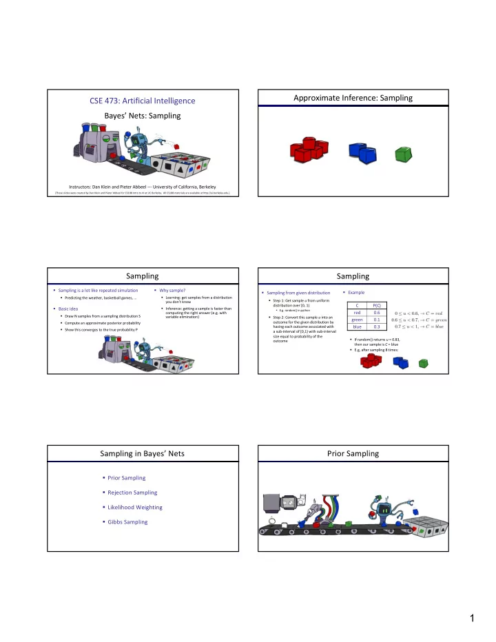§ Sampling from given distribution § Example § Predicting the weather, basketball games, … § Learning: get samples from a distribution § Step 1: Get sample u from uniform you don’t know distribution over [0, 1) C P(C) § Basic idea § Inference: getting a sample is faster than § E.g. random() in python red 0.6 computing the right answer (e.g. with § Draw N samples from a sampling distribution S variable elimination) § Step 2: Convert this sample u into an green 0.1 outcome for the given distribution by § Compute an approximate posterior probability having each outcome associated with blue 0.3 § Show this converges to the true probability P a sub-interval of [0,1) with sub-interval size equal to probability of the § If random() returns u = 0.83, outcome then our sample is C = blue § E.g, after sampling 8 times: Sampling in Bayes’ Nets Prior Sampling § Prior Sampling § Rejection Sampling § Likelihood Weighting § Gibbs Sampling 1

Prior Sampling Prior Sampling § For i=1, 2, …, n +c 0.5 -c 0.5 § Sample x i from P(X i | Parents(X i )) Cloudy Cloudy +c +s 0.1 +c +r 0.8 § Return (x 1 , x 2 , …, x n ) -s 0.9 -r 0.2 -c +s 0.5 -c +r 0.2 Sprinkler Sprinkler Rain Rain -s 0.5 -r 0.8 Samples: WetGrass WetGrass +w 0.99 +s +r -w 0.01 +c, -s, +r, +w -r +w 0.90 -c, +s, -r, +w -w 0.10 … +r +w 0.90 -s -w 0.10 -r +w 0.01 -w 0.99 Prior Sampling Example § This process generates samples with probability: § We ’ ll get a bunch of samples from the BN: C +c, -s, +r, +w +c, +s, +r, +w S R -c, +s, +r, -w …i.e. the BN ’ s joint probability W +c, -s, +r, +w -c, -s, -r, +w § Let the number of samples of an event be § If we want to know P(W) § We have counts <+w:4, -w:1> § Then § Normalize to get P(W) = <+w:0.8, -w:0.2> § This will get closer to the true distribution with more samples § Can estimate anything else, too § What about P(C| +w)? P(C| +r, +w)? P(C| -r, -w)? § I.e., the sampling procedure is consistent § Fast: can use fewer samples if less time (what’s the drawback?) Rejection Sampling Rejection Sampling § Let ’ s say we want P(C) § No point keeping all samples around § Just tally counts of C as we go C § Let ’ s say we want P(C| +s) S R § Same thing: tally C outcomes, but W ignore (reject) samples which don ’ t have S=+s +c, -s, +r, +w § This is called rejection sampling +c, +s, +r, +w § It is also consistent for conditional -c, +s, +r, -w +c, -s, +r, +w probabilities (i.e., correct in the limit) -c, -s, -r, +w 2

Rejection Sampling Likelihood Weighting IN: evidence instantiation § For i=1, 2, …, n § § Sample x i from P(X i | Parents(X i )) § If x i not consistent with evidence § Reject: Return, and no sample is generated in this cycle § Return (x 1 , x 2 , …, x n ) Likelihood Weighting Likelihood Weighting § Problem with rejection sampling: § Idea: fix evidence variables and sample the +c 0.5 rest -c 0.5 § If evidence is unlikely, rejects lots of samples § Evidence not exploited as you sample § Problem: sample distribution not consistent! Cloudy Cloudy § Consider P(Shape|blue) § Solution: weight by probability of evidence given parents +c +s 0.1 +c +r 0.8 pyramid, blue -s 0.9 -r 0.2 pyramid, green -c +s 0.5 -c +r 0.2 pyramid, red pyramid, blue Sprinkler Sprinkler Rain Rain -s 0.5 -r 0.8 sphere, blue sphere, blue Shape Color Shape Color cube, red cube, blue sphere, blue sphere, green Samples: WetGrass WetGrass +s +r +w 0.99 -w 0.01 +c, +s, +r, +w +w 0.90 -r … -w 0.10 +r +w 0.90 -s -w 0.10 -r +w 0.01 -w 0.99 Likelihood Weighting Likelihood Weighting § IN: evidence instantiation w = 1.0 § § Sampling distribution if z sampled and e fixed evidence for i=1, 2, …, n § § if X i is an evidence variable Cloudy C § X i = observation x i for X i § Set w = w * P(x i | Parents(X i )) S R § Now, samples have weights § else § Sample x i from P(X i | Parents(X i )) W § return (x 1 , x 2 , …, x n ), w § Together, weighted sampling distribution is consistent 3

Likelihood Weighting Gibbs Sampling § Likelihood weighting is good § Likelihood weighting doesn’t solve all our problems § We have taken evidence into account as we generate the sample § Evidence influences the choice of downstream E.g. here, W ’ s value will get picked based on the variables, but not upstream ones (C isn’t more § likely to get a value matching the evidence) evidence values of S, R § More of our samples will reflect the state of the § We would like to consider evidence when we world suggested by the evidence sample every variable à Gibbs sampling Gibbs Sampling Gibbs Sampling Example: P( S | +r) § Step 1: Fix evidence § Step 2: Initialize other variables C C § Procedure: keep track of a full instantiation x 1 , x 2 , …, x n . Start with an § R = +r § Randomly arbitrary instantiation consistent with the evidence. Sample one variable S +r S +r at a time, conditioned on all the rest, but keep evidence fixed. Keep repeating this for a long time. W W § Property: in the limit of repeating this infinitely many times the resulting § Steps 3: Repeat sample is coming from the correct distribution § Choose a non-evidence variable X § Resample X from P( X | all other variables) § Rationale : both upstream and downstream variables condition on evidence. C C C C C C § In contrast: likelihood weighting only conditions on upstream evidence, S +r S +r S +r S +r S +r S +r and hence weights obtained in likelihood weighting can sometimes be W W W W W W very small. Sum of weights over all samples is indicative of how many “effective” samples were obtained, so want high weight. Gibbs Sampling Efficient Resampling of One Variable § How is this better than sampling from the full joint? § Sample from P(S | +c, +r, -w) C § In a Bayes’ Net, sampling a variable given all the other variables (e.g. S +r P(R|S,C,W)) is usually much easier than sampling from the full joint W distribution § Only requires a join on the variable to be sampled (in this case, a join on R) § The resulting factor only depends on the variable’s parents, its children, and its children’s parents (this is often referred to as its Markov blanket) § Many things cancel out – only CPTs with S remain! § More generally: only CPTs that have resampled variable need to be considered, and joined together 4

Bayes’ Net Sampling Summary Further Reading on Gibbs Sampling* § Prior Sampling P § Rejection Sampling P( Q | e ) § Gibbs sampling produces sample from the query distribution P( Q | e ) in limit of re-sampling infinitely often § Gibbs sampling is a special case of more general methods called Markov chain Monte Carlo (MCMC) methods § Likelihood Weighting P( Q | e) § Gibbs Sampling P( Q | e ) § Metropolis-Hastings is one of the more famous MCMC methods (in fact, Gibbs sampling is a special case of Metropolis-Hastings) § You may read about Monte Carlo methods – they’re just sampling How About Particle Filtering? Particle Filtering X 1 X 2 X 2 = likelihood weighting § Particle filtering operates on ensemble of samples E 2 § Performs likelihood weighting for each individual sample to elapse time and incorporate evidence Elapse Weight Resample § Resamples from the weighted ensemble of samples to focus computation for the next time step where most of the probability mass is estimated to be Particles: Particles: Particles: (New) Particles: (3,3) (3,2) (3,2) w=.9 (3,2) (2,3) (2,3) (2,3) w=.2 (2,2) (3,3) (3,2) (3,2) w=.9 (3,2) (3,2) (3,1) (3,1) w=.4 (2,3) (3,3) (3,3) (3,3) w=.4 (3,3) (3,2) (3,2) (3,2) w=.9 (3,2) (1,2) (1,3) (1,3) w=.1 (1,3) (3,3) (2,3) (2,3) w=.2 (2,3) (3,3) (3,2) (3,2) w=.9 (3,2) (2,3) (2,2) (2,2) w=.4 (3,2) 5