Monte Carlo Methods Lecture slides for Chapter 17 of Deep Learning - PowerPoint PPT Presentation
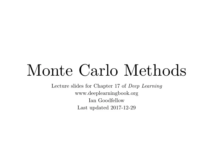
Monte Carlo Methods Lecture slides for Chapter 17 of Deep Learning www.deeplearningbook.org Ian Goodfellow Last updated 2017-12-29 Roadmap Basics of Monte Carlo methods Importance Sampling Markov Chains (Goodfellow 2017) Randomized
Monte Carlo Methods Lecture slides for Chapter 17 of Deep Learning www.deeplearningbook.org Ian Goodfellow Last updated 2017-12-29
Roadmap • Basics of Monte Carlo methods • Importance Sampling • Markov Chains (Goodfellow 2017)
Randomized Algorithms Las Vegas Monte Carlo Type of Random amount Exact Answer of error Chosen by user Random (until Runtime (longer runtime answer found) gives lesss error) (Goodfellow 2017)
Estimating sums / integrals with samples X X s = p ( x ) f ( x ) = E p [ f ( x )] (17.1) x Z s = p ( x ) f ( x ) d x = E p [ f ( x )] (17.2) to estimate, rewritten as an expectation, with the constraint n s n = 1 X f ( x ( i ) ) . ˆ (17.3) n i =1 (Goodfellow 2017)
Justification • Unbiased: • The expected value for finite n is equal to the correct value • The value for any specific n samples will have random error, but the errors for di ff erent sample sets cancel out • Low variance: • Variance is O (1/ n ) • For very large n , the error converges “almost surely” to 0 (Goodfellow 2017)
Roadmap • Basics of Monte Carlo methods • Importance Sampling • Markov Chains (Goodfellow 2017)
X Non-unique decomposition Z s = p ( x ) f ( x ) d x = E p [ f ( x )] (17.2) to estimate, rewritten as an expectation, with the constraint Say we want to compute Z a ( x ) b ( x ) c ( x ) d x . Which part is p ? Which part is f ? p = a and f =b c ? p = ab and f =c? etc. No unique decomposition. We can always pull part of any p into f. (Goodfellow 2017)
Importance Sampling p ( x ) f ( x ) = q ( x ) p ( x ) f ( x ) (17.8) , q ( x ) This ratio is our new f , This is our new p , meaning we will evaluate meaning it is the it at each sample distribution we will draw samples from (Goodfellow 2017)
Why use importance sampling? • Maybe it is feasible to sample from q but not from p • This is how GANs work • A good q can reduce the variance of the estimate • Importance sampling is still unbiased for every q (Goodfellow 2017)
Optimal q q ∗ ( x ) = p ( x ) | f ( x ) | , (17.13) Z • Determining the optimal q requires solving the original integral, so not useful in practice • Useful to understand intuition behind importance sampling • This q minimizes the variance • Places more mass on points where the weighted function is larger (Goodfellow 2017)
Roadmap • Basics of Monte Carlo methods • Importance Sampling • Markov Chains (Goodfellow 2017)
Sampling from p or q • So far we have assumed we can sample from p or q easily • This is true when p or q has a directed graphical model representation • Use ancestral sampling • Sample each node given its parents, moving from roots to leaves (Goodfellow 2017)
Sampling from undirected models • Sampling from undirected models is more di ffi cult • Can’t get a fair sample in one pass • Use a Monte Carlo algorithm that incrementally updates samples, comes closer to sampling from the right distribution at each step • This is called a Markov Chain (Goodfellow 2017)
Simple Markov Chain: Gibbs sampling • Repeatedly cycle through all variables • For each variable, randomly sample that variable given its Markov blanket • For an undirected model, the Markov blanket is just the neighbors in the graph • Block Gibbs trick: conditionally independent variables may be sampled simultaneously (Goodfellow 2017)
Gibbs sampling example • Initialize a, s, and b a s b • For n repetitions (a) • Sample a from P(a|s) and b from P(b|s) • Sample s from P(s|a,b) Block Gibbs trick lets us sample a and b in parallel (Goodfellow 2017)
Equilibrium • Running a Markov Chain long enough causes it to mix • After mixing, it samples from an equilibrium distribution • Sample before update comes from distribution π ( x ) • Sample after update is a di ff erent sample, but still from distribution π ( x ) (Goodfellow 2017)
Downsides • Generally infeasible to… • …know ahead of time how long mixing will take • …know how far a chain is from equilibrium • …know whether a chain is at equilibrium • Usually in deep learning we just run for n steps, for some n that we think will be big enough, and hope for the best (Goodfellow 2017)
Trouble in Practice • Mixing can take an infeasibly long time • This is especially true for • High-dimensional distributions • Distributions with strong correlations between variables • Distributions with multiple highly separated modes (Goodfellow 2017)
Di ffi cult Mixing Figure 17.1: Paths followed by Gibbs sampling for three distributions, with the Markov chain initialized at the mode in both cases. (Left) A multivariate normal distribution with two independent variables. Gibbs sampling mixes well because the variables are independent. (Center) A multivariate normal distribution with highly correlated variables. The correlation between variables makes it di ffi cult for the Markov chain to mix. Because the update for each variable must be conditioned on the other variable, the correlation reduces the rate at which the Markov chain can move away from the starting point. (Right) A mixture of Gaussians with widely separated modes that are not axis aligned. Gibbs sampling mixes very slowly because it is di ffi cult to change modes while altering only one variable at a time. (Goodfellow 2017)
Di ffi cult Mixing in Deep Generative Models Figure 17.2: An illustration of the slow mixing problem in deep probabilistic models. Each panel should be read left to right, top to bottom. (Left) Consecutive samples from Gibbs sampling applied to a deep Boltzmann machine trained on the MNIST dataset. Consecutive samples are similar to each other. Because the Gibbs sampling is performed in a deep graphical model, this similarity is based more on semantic than raw visual features, but it is still di ffi cult for the Gibbs chain to transition from one mode of the distribution to another, for example, by changing the digit identity. (Right) Consecutive ancestral samples from a generative adversarial network. Because ancestral sampling generates each sample independently from the others, there is no mixing problem. (Goodfellow 2017)
For more information… (Goodfellow 2017)
Recommend
More recommend
Explore More Topics
Stay informed with curated content and fresh updates.
