1 Example: Full Adder Diagnosis Inferring Solutions Example: Full - - PDF document

1

Diagnosis using Bounded Search Diagnosis using Bounded Search and Symbolic Inference and Symbolic Inference

Martin Sachenbacher and Brian C. Williams MIT CSAIL

Overview Overview

Soft Constraints Framework Characterizing Structure in Soft Constraints Exploiting Structure in Soft Constraints

– Set-based Search – Decomposition-based Search – Hybrids

Overview Overview

Soft Constraints Framework Characterizing Structure in Soft Constraints Exploiting Structure in Soft Constraints

– Set-based Search – Decomposition-based Search – Hybrids

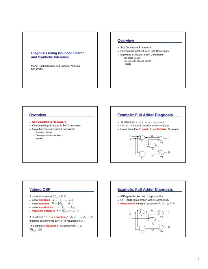
Example: Full Adder Diagnosis Example: Full Adder Diagnosis

Variables

• describe modes of gates

Gates are either in good ( ) or broken ( ) mode

Valued CSP Valued CSP

A constraint network

set of variables set of domains set of constraints valuation structure

A constraint is a function mapping assignments over to valuations in . The complete valuation of an assignment is .

Example: Full Adder Diagnosis Example: Full Adder Diagnosis

AND-gates broken with 1% probability OR-, XOR-gates broken with 5% probability Probabilistic valuation structure

2

Example: Full Adder Diagnosis Example: Full Adder Diagnosis

Model gates as soft constraints

Gate is good Gate is broken

Inferring Solutions Inferring Solutions

Constraint network Value of optimal solution obtained by combining the

constraints: Time: O(exp(n)) Space: O(exp(n))

Branch Branch-

• and

and-

• Bound Search

Bound Search

Lower Bound (lb):

Optimistic estimate of best solution in subtree

Each search node is a soft

constraint subproblem

Upper Bound (ub):

Best solution found so far

Prune, if lb ≥ ub.

Time: O(exp(n)) Space: O(n)

Overview Overview

Soft Constraints Framework Characterizing Structure in Soft Constraints Exploiting Structure in Soft Constraints

– Set-based Search – Decomposition-based Search – Hybrids

Structure in Soft Constraints Structure in Soft Constraints

Structure can be characterized as independence

properties of functions .

“Strong” independence: Function independent of

all assignments to some variables .

“Weak” independence: Function independent of

some assignments to some variables . Strong Weak

Strong Independence Strong Independence

Support

Subset of variables that function depends upon.

3

Strong Independence Strong Independence Strong Independence Strong Independence

Hypergraph

Weak Independence Weak Independence

E.g. for constraint : if , then value is

regardless of and Sharing of common subassignments.

Weak Independence Weak Independence Weak Independence Weak Independence

Algebraic Decision Diagram

Overview Overview

Soft Constraints Framework Characterizing Structure in Soft Constraints Exploiting Structure in Soft Constraints

– Decomposition-based Search – Set-based Search – Hybrids

4

Exploiting Strong Independence Exploiting Strong Independence

Principle: Strong independence allows to

decompose the problem into subproblems with smaller sets of variables.

Tree Decomposition Tree Decomposition

Subproblems

Tree Decomposition Tree Decomposition

Constraints λ Variables χ

BnB with Tree Decomposition BnB with Tree Decomposition

Algorithm BTD (Terrioux and Jégou CP-03) Record solutions for subproblems (“structural goods”)

BnB with Tree Decomposition BnB with Tree Decomposition

Algorithm BTD (Terrioux and Jégou CP-03) Record solutions for subproblems (“structural goods”)

Time: O(exp(maxi|χi|)) Space: O(exp(maxi,j|χi-χj|))

EO EO-

• 1 Model: Constraint Graph

1 Model: Constraint Graph

5

EO EO-

• 1 Model: Tree Decomposition

1 Model: Tree Decomposition Ssa2670 Ssa2670-

• 141 Circuit: Graph

141 Circuit: Graph Ssa2670 Ssa2670-

• 130 Circuit: Tree

130 Circuit: Tree Overview Overview

Soft Constraints Framework Characterizing Structure in Soft Constraints Exploiting Structure in Soft Constraints

– Decomposition-based Search – Set-based Search – Hybrids

Exploiting Weak Independence Exploiting Weak Independence

Principle: Weak independence allows to consider

sets of assignments at once instead of individual assignments.

Set Set-

• based Branch

based Branch-

• and

and-

• Bound

Bound

Lower Bound Function

(flb): Optimistic estimates

• f best solutions in subtree

Each search node is a set of

soft constraint subproblems

Upper Bound (ub):

Best solution found so far

Prune, if flb ≥ ub.

Encode e.g. using ADD

6

Domain Splitting Domain Splitting

Generalize to search over sets:

Partition domains into sets Choose subset

for unassigned variable

Example: 4 Example: 4-

• Queens

Queens

Variables: Rows Domains: Columns Constraints:

Q Q Q Q

Example Example

Search Tree

Solution

Example Example

Domain splitting with partitions

Solution

Example Example

Domain splitting with partitions

Solution

Results Results

C++ Implementation of SBBTD on Pentium 4 with 1

GB RAM, using ADD library from CUDD package

Weighted version of 16-Queens-Problem (16

variables, 136 constraints, domain size 16)

Using partition {{0,...,15}}: out of memory (> 1 GB) Using partition {{0},{1},…, {15}}: out of time (>10 min) Using partition {{0,...,7},{8,...,15}}: 104.8 sec

7

Overview Overview

Soft Constraints Framework Characterizing Structure in Soft Constraints Exploiting Structure in Soft Constraints

– Set-based Search – Decomposition-based Search – Hybrids

Hybrid Algorithm SBBTD Hybrid Algorithm SBBTD

Exploits both strong independence using tree

decomposition, and weak independence using set- based search.

SBBTD applied to Full Adder SBBTD applied to Full Adder

Partition , all else

SBBTD applied to Full Adder SBBTD applied to Full Adder

Search Tree

Upper bound = 0

SBBTD applied to Full Adder SBBTD applied to Full Adder

Search Tree

<u=0, y=0> .047 <u=0, y=1> .902 Upper bound = 0

SBBTD applied to Full Adder SBBTD applied to Full Adder

Search Tree

<u=0, y=0> .047 <u=0, y=1> .902 <v=0, w=0> .950 Upper bound = .044

8

SBBTD applied to Full Adder SBBTD applied to Full Adder

Search Tree

<u=0, y=0> .047 <u=0, y=1> .902 <v=0, w=0> .950 Upper bound = .044

SBBTD applied to Full Adder SBBTD applied to Full Adder

Search Tree

<u=0, y=0> .047 <u=0, y=1> .902 <v=0, w=0> .950 Upper bound = .044 Exploiting goods recorded at v2 (“forward jump”)

SBBTD applied to Full Adder SBBTD applied to Full Adder

Search Tree

<u=0, y=0> .047 <u=0, y=1> .902 <v=0, w=0> .950 <v=0, w=1> .050 Upper bound = .044

SBBTD applied to Full Adder SBBTD applied to Full Adder

Search Tree

<u=0, y=0> .047 <u=0, y=1> .902 <v=0, w=0> .950 <v=0, w=1> .050 Upper bound = .044 Cut by bound

SBBTD applied to Full Adder SBBTD applied to Full Adder

Search Tree

Cut by bound

SBBTD applied to Full Adder SBBTD applied to Full Adder

Search Tree

Cut by bound

9

SBBTD applied to Full Adder SBBTD applied to Full Adder

Search Tree

Cut by bound

SBBTD applied to Full Adder SBBTD applied to Full Adder

Search Tree

Cut by bound

SBBTD applied to Full Adder SBBTD applied to Full Adder

Search Tree

Cut by bound Finished. Best solution = .044 # Nodes = 45

Results Results

C++ Implementation of SBBTD on Pentium 4 with 1

GB RAM, using ADD library from CUDD package

Weighted version of ssa0432-003 circuit (435

variables, 1027 constraints, domain size 2)

Time to compute tree decomposition: 5 sec. Using partition {{0},{1}}: out of time (>10 min) Using partition {{0,1}}: 3 sec.

Future Work Future Work

Determine optimal granularity of domain partitions? Combination with local filtering techniques?

Material Material

Material

10

Main Idea Main Idea

Diagnosis as soft constraint solving (DX-2004) Efficient techniques for solving soft constraints? Branch-and-Bound Search: memory efficient, but

time exponential (backtracking)

Inference: no backtracking, but memory exponential Techniques to exploit structure: Decision diagrams,

Tree Decompositions

Still memory exponential. Idea: hybrid of branch-and-bound search, symbolic

encoding and tree decomposition.

Soft Soft CSPs CSPs

Unified framework for constraints and preferences. For each constraint/tuple, a valuation that reflects

preference (e.g. cost, weight, priority, probability, …).

The valuation of an assignment is the combination

• f the valuations for each constraint, using a binary
• perator (with special axioms).

Assignments are compared using a total order on

valuations.

The problem is to produce an assignment of

minimum valuation.

Formally: Valuation Structure Formally: Valuation Structure

• = set of valuations, used to assess assignments
• = minimum element of , corresponds to totally

consistent assignments

• = maximum element of , corresponds to totally

inconsistent assignments

• = total order on E, used to compare two valuations
• = operator used to combine two valuations

(commutative, associative, monotonic, neutral element , annihilator )

Decision Diagrams Decision Diagrams

Example

Binary Decision Trees Binary Decision Trees

Recursive Shannon expansion

x 1 y 1 z 1 1 1 1 z z y y 1 1 1 1

Variable Ordering Variable Ordering

Impose arbitrary total ordering on variables Variables must obey ordering along all paths Property: No conflicting assignments along path

x y z x y z y x x x

11

Ordered Binary Decision Tree Ordered Binary Decision Tree

Order

x y y 1 1 1 1 z z z z 1 1 1 1 1 1

Ordered Binary Decision Tree Ordered Binary Decision Tree

x y y 1 1 1 1 z z z z 1 1 1 1 1 1

Rule 1: Collapse Leaf Nodes Rule 1: Collapse Leaf Nodes

x y y 1 1 1 z z z z 1 1 1 1 1 No longer a tree.

Rule 2: Remove Redundant Tests Rule 2: Remove Redundant Tests

x y y 1 1 1 z z z 1 1 1 1 z 1

Rule 2: Remove Redundant Tests Rule 2: Remove Redundant Tests

x y y 1 1 1 z z z 1 1 1 1

Rule 3: Isomorphic Rule 3: Isomorphic Subgraphs Subgraphs

x y y 1 1 1 z 1 1 z z 1 1

12

Rule 3: Isomorphic Rule 3: Isomorphic Subgraphs Subgraphs

x y y 1 1 1 z 1 1

Rule may become applicable again Rule may become applicable again

x y 1 1 y 1 z 1 1

Final Representation Final Representation

x y 1 1 z 1 1 Reduced, Ordered Binary Decision Diagram (ROBDD)

ROBDDs ROBDDs

Contains only variables from support Time and space complexity of operations depends

• n ROBDD size rather than number of assignments

Can be extended to functions with non-binary values

and non-binary variables

– Algebraic Decision Diagrams (ADDs) [Bahar et al. 93] – Multi-valued Decision Diagram (MDDs) [Kam 90]

Significant compaction in many practical cases.

Example Example

Full Adder

Tree Decomposition Tree Decomposition

Every variable of the original problem must appear in

at least one subproblem.

Every constraint of the original problem must appear

in a subproblem, along with all variables in its scope (covering condition).

If a variable occurs in two subproblems, it must

appear in every subproblem along the path that connects the two (connectedness condition).

13

Example: Full Adder Example: Full Adder

Constraints Variables

Tree Decomposition Tree Decomposition

Principle: Solve each subproblem, then combine

solutions using dynamic programming.

Time O(exp(tw)), where tree width tw is maximum

number of variables in a subproblem minus one.

Space O(exp(sw)), where separator width sw is

maximum number of variables shared between subproblems.

Finding decompositions with minimal width is NP-

hard, but good heuristics exist.

The width is often small in practice.

BTD ( BTD (Terrioux Terrioux and and J Jé égou gou CP CP-

• 03)

03)

Assign variables in subproblem, beginning with root

• f the tree decomposition.

Inside a subproblem, use classical branch-and-

bound, considering only the constraints of the subproblem.

Once all variables in the subproblem have been

assigned, consider its children (if any).

Given a child, check if the current assignment,

restricted to variables shared with the child, has been previously recorded as a good.

BTD ( BTD (Terrioux Terrioux and and J Jé égou gou CP CP-

• 03)

03)

If it is not previously recorded, compute solution for

the subproblem given the current assignment and upper bound, and record it as new good.

Add recorded value to value of current assignment. If resulting value is below the upper bound, proceed

with the next child, else backtrack.

Projection Projection

• ,

Combination Combination

14

Combination Combination

• Soft

Soft CSPs CSPs

For each constraint/tuple: a valuation that reflects

preference (e.g. cost, weight, probability, …).

Valuations are combined using a binary operator

(with special axioms).

Assignments are compared using a total order on

valuations.

The problem is to produce an assignment of

minimum valuation.

Sinking Operation Sinking Operation

• is a new constraint where all values of

tuples have been replaced by

Generalizes the test to functions

Constraint sink(fe2,0.05) Constraint

Set Set-

• based Branch

based Branch-

• and

and-

• Bound

Bound

Function

( : assignments, : value): value if then if then return let be an unassigned variable for each do return return Time: O(exp(n)) Space: O(exp(n))

Branch Branch-

• and

and-

• Bound Search

Bound Search

Function

( : assignment, : value): value if then if then return let be an unassigned variable for each do return return Time: O(exp(n)) Space: O(n)