1 Sampling error The long term average value for p is 0.5; lets call - - PDF document

1

Population Genetics 1: Genetic Drift

( ) ( )

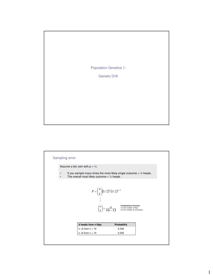
k n k

k n P

−

⎟ ⎟ ⎠ ⎞ ⎜ ⎜ ⎝ ⎛ = 2 / 1 2 / 1

( )

! ! ! k n k n k n − = ⎟ ⎟ ⎠ ⎞ ⎜ ⎜ ⎝ ⎛

Combinations Formula: n is the number of flips k is the number of successes

Assume a fair coin with p = ½:

• If you sample many times the most likely single outcome = ½ heads.
• The overall most likely outcome ≠ ½ heads

0.205 k =6 from n = 10 0.246 k =5 from n = 10 Probability k heads from n flips

Sampling error

2

0.005 0.002 0.16 0.68 0.16 0.002 50 0.0125 0.06 0.19 0.50 0.19 0.06 20 0.025 0.16 0.21 0.25 0.21 0.16 10

variance p <0.65 p = 0.55-0.65 p = 0.45-0.55 p = 0.35-0.45 p <0.35 N flips

Sampling error

The long term average value for p is 0.5; let’s call that E(p). How do we improve our changes of getting something close E(p)? If we flipped the coin 1000 times: we get very close to E(p) in a single try, but not exactly.

Genetic drift

Consider a diploid population:

• Ideal population: no sampling errors because infinite population size
• Natural population: finite size and finite sample of gametes [errors]

Example: Let’s assume: A = p = 0.75; a = q = 0.25; N = 500 This generation: 200 individuals reproduce [400 gametes] This is a binomial sampling problem: The probability of getting p = 0.75 and q = 0.25 in next generation is: P = 0.046

( ) ( )

100 300

25 . 75 . 300 400 ⎟ ⎟ ⎠ ⎞ ⎜ ⎜ ⎝ ⎛ = P

3

Draw 4:6 Draw 7:3 Draw 8:2 Restock Restock Restock Generation 0 Generation 1 Generation 2 Generation 3 white = 0.5 white = 0.4 white = 0.7 white = 0.8 Draw 4:6 Draw 7:3 Draw 8:2 Restock Restock Restock Generation 0 Generation 1 Generation 2 Generation 3 white = 0.5 white = 0.4 white = 0.7 white = 0.8

Genetic drift

Genetic drift is the accumulation of random sampling fluctuations in allele frequencies over generations.

N 1

e

1N Genetic drift

The magnitude of change in allele frequencies is inversely proportional to the sample size:

Ideal population with finite size and finite gamete sample per

• generation. See last slide for

example

Remember that natural populations are less than ideal in many more ways! In most natural populations the effective size (Ne) will be less than the census size. The magnitude of drift in natural populations is: Drift and inbreeding effects are not independent!

4

Ne = 100 Ne = 1000 Ne = 10000 Ne = 50000

Genetic drift Genetic drift

• rate to fixation [under drift] slows with increasing in Ne
• ultimate fate is fixation of loss

If we run this simulation long enough it will go to fixation of loss; it just takes much longer

5

Genetic drift

What is the fate (on average) of a new mutant?

e

1N

The probability of fixation of a new mutant is its frequency (p or q) in the population: This is al low as it gets. The fate of most new mutations is LOSS due to drift.

WAA = 0.5; WAa = 0.5; Waa = 1:

• ideal population: probability of fixation = 1
• population with Ne = 50: probability of fixation ~ 0.25

Probability of fixation actually declines as Ne increases!

. 2 . 4 . 6 . 8 1 1 3 5 7 9 11 13 15 17 19 21 23 25 . 2 . 4 . 6 . 8 1 1 3 5 7 9 11 13 15 17 19 21 23 25 . 2 . 4 . 6 . 8 1 1 3 5 7 9 11 13 15 17 19 21 23 25 . 1 . 2 . 3 . 4 . 5 . 6 . 7 . 8 . 9 1 1 3 5 7 9 11 13 15 17 19 21 23 25 . 2 . 4 . 6 . 8 1 1 3 5 7 9 11 13 15 17 19 21 23 25 . 2 . 4 . 6 . 8 1 1 3 5 7 9 11 13 15 17 19 21 23 25 . 2 . 4 . 6 . 8 1 1 3 5 7 9 11 13 15 17 19 21 23 25 . 2 . 4 . 6 . 8 1 1 3 5 7 9 11 13 15 17 19 21 23 25 . 2 . 4 . 6 . 8 1 1 3 5 7 9 11 13 15 17 19 21 23 25 . 2 . 4 . 6 . 8 1 1 3 5 7 9 11 13 15 17 19 21 23 25

Generation Allele frequency

* * * = fixation

Genetic drift Changes in allele frequency due to drift are unpredictable! Note if we ran more generations, more popns would go to fixation

10 Independent populations; each started with p = q = 0.5 Ne = 50; generations = 50

6

5 10 15 20 25 1 2 3 4 5 6 7 8 9 10 11 12 13 5 10 15 20 25 30 35 40 45 1 2 3 4 5 6 7 8 9 10 11 12 13

0 allele frequency 1 0 allele frequency 1 number of populations

initial distribution; t = 0 generations distribution after t = 50 generations

Genetic drift Genetic drift

The effects of drift are cumulative over time. The effects of drift are predictable as averaged over time and populations: 1. loss of variation within populations 2. gain in variation between populations

7

Let x be the amount of change in p and q a population due to drift. As we have seen the long term average, E(x), due to drift will be zero because changes in p and q are equally likely to be positive or negative. Given E(x) = 0, what happens to heterozygosity? Does heterozygosity change at all?

Does genetic drift affects heterozygosity?

Let’s start with HW at generation t: Ht = 2pq The allele frequencies, p and q, will change from generation to generation by the amount x: Ht+1 = 2(p + x)(q – x) Ht+1 = 2pq + 2x(q – p) – 2x2 Although E(x) = 0, the expected value of x-squared, E(x2), is always positive. E(2pq + 2x(q – p) – 2x2) 2pq – 2x2 Heterozygosity is expected reduced by genetic drift. Nice, eh?

Genetic drift and inbreeding are not independent

• 1. Unequal numbers in successive generations

(approx.) 1 ... 1 1 1 1 1

3 2 1

⎥ ⎥ ⎦ ⎤ ⎢ ⎢ ⎣ ⎡ + + + + =

g e

N N N N g N

• 2. Different numbers of males and females

(approx.) 4 1 4 1 1

f m e

N N N + =

• 3. Variance in reproductive success (other than male verse female)

( )

2 2 4 + − =

k v e

V N N

8

Bottlenecks and founder effects Bottleneck: is a single, extraordinarily large, reduction in population size

Pre-bottleneck population Post-bottleneck population Bottleneck event

1. Change in allele frequencies, as compared with pre-bottleneck population 2. Reduction in diversity

Bottlenecks and founder effects

Effective population size is dominated by historical lows and can be very much lower than current

census size. 20,000 40,000 60,000 80,000 100,000 120,000 1 2 3 4 5 6 7 8 9 10 11 12 13 14 15 16 17 18 19 20 21 22 23 24 Time population census size Ave N Ne

Population crash Population recovered to historical high

(approx.) 1 ... 1 1 1 1 1

3 2 1

⎥ ⎥ ⎦ ⎤ ⎢ ⎢ ⎣ ⎡ + + + + =

g e

N N N N g N

9

Parental population Dispersal event to a neighbouring island Island 1 New population Island 2

Two species that have suffered extreme bottlenecks due to commercial harvesting

Northern right whale Poor population recovery Northern elephant seal Excellent population recovery

10

Keynotes:

• Genetic drift influences allele frequency and genotype frequency.
• Drift decreases diversity within populations and increases diversity between

populations.

• Under drift, fixation rate is determined by Ne; the probability of fixation by p.
• In specific cases the outcome of genetic drift is unpredictable.
• The effects of drift are predictable as an average over populations.
• Drift might reduce a population’s ability to evolve in response to new selective

pressures (remember Trudy MacKay’s experiments). Alternatively, some believe that drift could actually increase the rate of speciation.

• Drift is particularly important in rare and endangered species.
• Founder effects may play an important role in some speciation events

Genetic drift

Acts on all loci in the genome; results in loss of heterozygosity and loss of alleles yes yes Genetic Drift Acts on the locus subject to selection, and those loci linked to it yes yes Natural Selection Very very very slow yes yes Mutation Depends of migration rate and frequency differences between populations yes yes Migration a Only acts on the locus subject to assortment, and those loci linked to it no yes Assortative Mating Acts on all loci in genome; results in loss of heterozygosity no yes Inbreeding Creates disequilibrium among loci no no Linkage Notes Allele Genotype Agency Change in frequencies

HW model: no change in frequencies Alt model; change in frequencies (molecular evolution)