1 Quantitative and Qualitative Divide and Conquer In this figure, - - PDF document

1

Iso-Contouring and Level-Sets

Roger Crawfis

Contributors: Roger Crawfis, Han-Wei Shen, Raghu Machiraju, Torsten Moeller, Fan Ding, Charles Dyer, and Huang Zhiyong

4/17/2003

• R. Crawfis, Ohio State Univ.

2

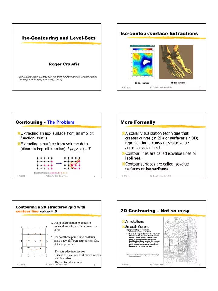
Iso-contour/surface Extractions

2D Iso-contour 3D Iso-surface

4/17/2003

• R. Crawfis, Ohio State Univ.

3

Contouring - The Problem

Extracting an iso- surface from an implicit function, that is, Extracting a surface from volume data (discrete implicit function), f (x ,y ,z ) = T

4/17/2003

• R. Crawfis, Ohio State Univ.

4

More Formally

A scalar visualization technique that creates curves (in 2D) or surfaces (in 3D) representing a constant scalar value across a scalar field. Contour lines are called isovalue lines or isolines. Contour surfaces are called isovalue surfaces or isosurfaces

4/17/2003

• R. Crawfis, Ohio State Univ.

5

Contouring a 2D structured grid with contour line value = 5

0 1 1 3 2 1 3 6 6 3 3 7 9 7 3 2 7 8 6 2 1 2 3 4 3

• 1. Using interpolation to generate

points along edges with the constant value

• 2. Connect these points into contours

using a few different approaches. One

• f the approaches:

. Detects edge intersection . Tracks this contour as it moves across cell boundary . Repeat for all contours

4/17/2003

• R. Crawfis, Ohio State Univ.

6

2D Contouring – Not so easy

Annotations Smooth Curves

Topographic Map of Jerusalem (Contour interval 10 meters) North is at the top of the map. The Mount of Olives is on the far right, Mount Zion on the left. Mount Moriah rises as a long ridge at the south end of the City of David and continues on past the present Temple Mount, and reaches its highest point outside the Northern walls of the Old City, at the top of the map.

http://www.skullandcrossbones.org/articles/solomontemple /solomontemple2.htm

2

4/17/2003

• R. Crawfis, Ohio State Univ.

7

Quantitative and Qualitative

In this figure, we can actually read off any value to about three significant digits. Hard and tedious problem to determine where to place labels. Usually done as vector graphics, rather than raster graphics for precision.

http://omnimap.com/catalog/cats/fish/fish-contour.htm

4/17/2003

• R. Crawfis, Ohio State Univ.

8

Divide and Conquer

Partition space into rectangular sub- regions.

4/17/2003

• R. Crawfis, Ohio State Univ.

9

Dividing Cubes/Squares

Generates Points and renders them Rendering points is faster than polygons Principle - Divide a square until contour passes thru the cell 1 2 3 4 3 2 7 8 6 2 3 7 9 7 3 1 3 6 6 3 1 1 3 2 Iso-value=5

4/17/2003

• R. Crawfis, Ohio State Univ.

10

Dividing Cubes

• 1. Create a cell
• 2. Determine if the cell is a surface cell
• 3. Subdivide surface cells to image resolution
• 4. Determine intensity or color of refined cell
• 5. Output a point for each remaining surface cell

4/17/2003

• R. Crawfis, Ohio State Univ.

11

Step 3: Subdivide

Subdivide each cell such that the resolution is higher than the image resolution. For example, when a 1282 volume is rendered to a 5122 image, cells containing the contour will be divided to 4x4x4 smaller cubes. classify subdivide

• utput points

4/17/2003

• R. Crawfis, Ohio State Univ.

12

Surface Tracking

Given function S(t,x,y,z) that returns 1 if (x,y,z) is on the surface t and 0

• therwise

Needed: a seed voxel p that is on the surface. 1 2 3 4 3 2 7 8 6 2 3 7 9 7 3 1 3 6 6 3 1 1 3 2 Iso-value=5 Seed cell

3

4/17/2003

• R. Crawfis, Ohio State Univ.

13

Surface Tracking

Let Q be a queue of voxels.

Push p onto Q Flag p as “visited” While Q is not empty do Pop q from Q and output it. For each voxel v in the neighborhood of q do If S(t, v) = 1 then If v was not visited then Push v onto Q Flag it as “visited” end {while}

4/17/2003

• R. Crawfis, Ohio State Univ.

14

Tracking and Smooth Curves

Recall that the gradient to a scalar field is normal to the isolines. Therefore, the curve will be towards the direction perpendicular to the gradient. Can also use the gradient to calculate tangents for each point on the curve to generate smooth curves.

4/17/2003

• R. Crawfis, Ohio State Univ.

15

Restricted Topological Cases

Filled circle vertices indicate scalar value is above the contour value Unfilled ones which scalar values are below the contour values

• A closed curve can not be contained in the cell.
• The curve can only enter and exit the cell once per edge.

4/17/2003

• R. Crawfis, Ohio State Univ.

16

Not Allowed

4/17/2003

• R. Crawfis, Ohio State Univ.

17

Linear Topology

The restricted set is topologically equivalent to linear segments. Topologically equivalent if we restrict the edge intersections to lie at the mid-points of each edge.

4/17/2003

• R. Crawfis, Ohio State Univ.

18

Using Symmetry to Reduce to 5

Contour ambiguity: either solid

• r dash lines look OK

4

4/17/2003

• R. Crawfis, Ohio State Univ.

19

2D Iso-contour (0)

Remember bi-linear interpolation

p2 p3 p0 p1 P =? p4 p5

To know the value of P, we can first compute p4 and P5 and then linearly interpolate P

4/17/2003

• R. Crawfis, Ohio State Univ.

20

2D Iso-contour (1)

Consider a simple case: one cell data set

The problem of extracting an iso-contour is an inverse of value interpolation. That is:

p2 p3 p0 p1 Given f(p0)=v0, f(p1)=v1, f(p2)=v2, f(p3)=v3 Find the point(s) P within the cell that have values F(p) = C

4/17/2003

• R. Crawfis, Ohio State Univ.

21

2D Iso-contour (2)

p2 p3 p0 p1

We can solve the problem based on linear interpolation

(1) Identify edges that contain points P that have value f(P) = C (2) Calculate the positions of P (3) Connect the points with lines

4/17/2003

• R. Crawfis, Ohio State Univ.

22

2D Iso-contouring – Step 1

(1) Identify edges that contain points P that have value f(P) = C

v1 v2 If v1 < C < v2 then the edge contains such a point

4/17/2003

• R. Crawfis, Ohio State Univ.

23

2D Iso-contouring – Step 2

(2) Calculate the position of P

Use linear interpolation: P = P1 + (C-v1)/(v2-v1) * (P2 – P1) v1 v2 P p1 p2 C

4/17/2003

• R. Crawfis, Ohio State Univ.

24

2D Iso-contouring – Step 3

p2 p3 p0 p1 Connect the points with line(s) Based on the principle of linear variation, all the points on the line have values equal C

5

4/17/2003

• R. Crawfis, Ohio State Univ.

25

Inside or Outside?

Just a naming convention

• 1. If a value is smaller than the iso-value, we call it “Outside”
• 2. If a value is greater than the iso-value, we call it “Inside”

p2 p3 p0 p1

• +

inside cell

p2 p3 p0 p1

• utside cell

4/17/2003

• R. Crawfis, Ohio State Univ.

26

Contouring in 3D

Treat volume as a set of 2D slices

Apply 2D Contouring algorithm on each slice. Or given as a set of hand-drawn contours

Stitch the slices together.

4/17/2003

• R. Crawfis, Ohio State Univ.

27

Contour Stitching

• Problem:

Problem: Given: 2 two Given: 2 two-

• dimensional

dimensional closed closed curves curves Curve #1 has Curve #1 has m m points points Curve #2 has Curve #2 has n n points points Which point(s) does vertex Which point(s) does vertex i i on curve one correspond to

• n curve one correspond to
• n curve two?
• n curve two?

? ? i

4/17/2003

• R. Crawfis, Ohio State Univ.

28

A Solution

Fuchs, et. al.

Optimization problem 1 stitch consists of:

⌧2 spans between curves ⌧1 contour segment

Triangles of {Pi,Qj,Pi+1} or {Qj+1,Pi,Qj}

⌧Consistent normal directions Pi Pi+1 Qj

4/17/2003

• R. Crawfis, Ohio State Univ.

29

Fuchs, et. al.

Left span

PiQj => go up

Right span (either)

Pi+1Qj => go down PiQj+1 => go down

4/17/2003

• R. Crawfis, Ohio State Univ.

30

Fuchs, et. al.

Constraints

Each contour segment is used once and only

• nce.

If a span appears as a left span, then it must also appear as a right span. If a span appears as a right span, then it must also appear as a left span.

6

4/17/2003

• R. Crawfis, Ohio State Univ.

31

Fuchs, et. al.

This produces an acceptable surface (from a topological point of view)

No holes

We would like an optimal one in some sense.

4/17/2003

• R. Crawfis, Ohio State Univ.

32

Fuchs et. al.

Graph problem Vertices Vij = span between Pi and Qj Edges are constructed from a left span to a right span.

Only two valid right spans for a left span.

P Pi

i

Q Qj

j

Q Qj+1

j+1

P Pi+1

i+1

4/17/2003

• R. Crawfis, Ohio State Univ.

33

Fuchs, et. al.

Organize these edges as a grid or matrix. P P Q Q

i j

PiQjPi+1 QjPiQj+1

4/17/2003

• R. Crawfis, Ohio State Univ.

34

Fuchs, et. al.

Acceptable graphs

Exactly one vertical arc between Pi and Pi+1 Exactly one horiz. arc between Qj and Qj+1 Either

⌧indegree(Vij) = outdegree(Vij) = 0 ⌧both > 0

• (if a right, also has to be a left)

4/17/2003

• R. Crawfis, Ohio State Univ.

35

Fuchs, et. al.

Claim:

An acceptable graph, S, is weakly connected.

Lemma 2

Only 0 or 1 vertex of S has an indegree = 2.

⌧E.g., Two cones touching in the center.

All other vertices have indegree=1 (recall indegree = outdegree)

4/17/2003

• R. Crawfis, Ohio State Univ.

36

Fuchs, et. al.

Thereom 1: S is an acceptable surface if and only if:

S has one and only one horizontal arc between adjacent columns. S has one and only one vertical arc between adjacent rows. S is Eulerian (closed walk with every arc only

• nce).

7

4/17/2003

• R. Crawfis, Ohio State Univ.

37

Fuchs, et. al.

Number of arcs is thus m+n. Many possible solutions still!!! Associate costs with each edge

Area of resulting triangle Aspect ratio of resulting triangle

4/17/2003

• R. Crawfis, Ohio State Univ.

38

Fuchs, et. al.

Note that Vi0 is in S for some i. Note that V0j is in S for some j. With the weights (costs), we can compute the minimum path from a starting node Vi0.

Since we do not know which Vi0, we compute the paths for all of them and take the minimum.

⌧Some cost saving are achievable.

4/17/2003

• R. Crawfis, Ohio State Univ.

39

Marching Cubes

Predominant method used today. Efficient and simple It was independently reported by Wyvill and McPeeters in 1986, Lorenson and Cline in 1987

4/17/2003

• R. Crawfis, Ohio State Univ.

40

Marching Cubes

Treat each cube individual

No 2D contour curves

Allow intersections only on the edges or at vertices. Pre-calculate all of the necessary information to construct a surface.

4/17/2003

• R. Crawfis, Ohio State Univ.

41

Marching Cubes

Consider a single cube

All vertices above the contour threshold All vertices below Mixed above and below

+ + + + + +

• +

4/17/2003

• R. Crawfis, Ohio State Univ.

42

Marching Cubes

Binary label each node => (above/below) Examine all possible cases

• f above or below for each

vertex. 8 vertices implies 256 possible cases.

+ + + + + +

• +

8

4/17/2003

• R. Crawfis, Ohio State Univ.

43

How many cases?

Now we have 8 vertices So it is: 2 = 256

8

How many unique topological cases?

4/17/2003

• R. Crawfis, Ohio State Univ.

44

Case Reduction

Value Symmetry

+ + _ _ _ _ _ _ + + _ _ + + + +

4/17/2003

• R. Crawfis, Ohio State Univ.

45

Case Reduction

Rotation Symmetry

+ + _ _ _ _ _ _ _ _ + + _ _ _ _

4/17/2003

• R. Crawfis, Ohio State Univ.

46

Case Reduction

Mirror Symmetry

+ + _ + _ + _ _ _ + + + + _ _ _ By inspection, we can reduce 256 14

4/17/2003

• R. Crawfis, Ohio State Univ.

47

Marching Cube - Summary

Create a cube Classify each voxel Build an index Lookup edge list Interpolate triangle vertices Calculate and interpolate normals

4/17/2003

• R. Crawfis, Ohio State Univ.

48

Step 1: Create a Cube

Consider a cube defined by eight data values: four from slice K, and four from slice K+ 1

9

4/17/2003

• R. Crawfis, Ohio State Univ.

49

Step 2: Classify Each Voxel

Binary classification of each vertex of the cube as to whether it lies

• utside the surface (voxel value < isosurface value)
• r inside the surface (voxel value <= isosurface

value).

4/17/2003

• R. Crawfis, Ohio State Univ.

50

Step 3: Build an Index

Use the binary labeling of each voxel to create an 8-bit index:

8 vertices - 256 cases Requires a canonical

• rdering of the cube.

4/17/2003

• R. Crawfis, Ohio State Univ.

51

Step 4: Look-up the Topology

Given the index for each cell, a table lookup is performed to identify the edges that has intersections with the iso-surface. Also requires a canonical ordering

• f the edges: e1, e2, …, e12

1 2 3 14 e1, e3, e5

…

Index intersection edges e1

e2

e3 e4

e5

e6 e7 e8 e9 e10 e11 e12

4/17/2003

• R. Crawfis, Ohio State Univ.

52

Step 4: Look-up the Topology

all 256 cases could be derived from 15 base cases. Difficult to determine rotational symmetry and map it correctly to the table.

4/17/2003

• R. Crawfis, Ohio State Univ.

53

Step 4: Example

Index = 10001101 triangle 1 = e4,e7,e12 triangle 2 = e1, e7, e4 triangle 3 = e1, e6, e7 triangle 4 = e1, e10, e6 e1 e10 e6 e7 e12 e4

v1 v2 v7

e2

4/17/2003

• R. Crawfis, Ohio State Univ.

54

Step 5: Interpolate Triangle Vertices

For each edge, find the vertex location along the edge using linear interpolation of the voxel values.

10

4/17/2003

• R. Crawfis, Ohio State Univ.

55

Step 6: Compute Normals

Calculate the normal at each cube vertex Use linear interpolation to interpolate the polygon vertex normal

4/17/2003

• R. Crawfis, Ohio State Univ.

56

Why is it called marching cubes?

Linear search through cells

• Row by row, layer by layer
• Reuse the interpolated points

for adjacent cells No neighborhood information No neighborhood information is required!!! is required!!!

4/17/2003

• R. Crawfis, Ohio State Univ.

57

Problems

Ambiguities: Are the curves below right or wrong?

4/17/2003

• R. Crawfis, Ohio State Univ.

58

Problems

Inconsistencies: Does the result produce the correct topology? An iso-contour surface should always be a manifold.

We know whether these cases are right or wrong.

wrong

4/17/2003

• R. Crawfis, Ohio State Univ.

59

2D Contouring Ambiguity

Break contour Join contour

• r

Either choices are acceptable because contour lines are continuous and closed Independent of other choices

4/17/2003

• R. Crawfis, Ohio State Univ.

60

Marching Cubes

Topological inconsistencies in the 15 cases

Turns out positive and negative are not symmetric.

+ + + + + +

• +
• +

+

11

4/17/2003

• R. Crawfis, Ohio State Univ.

61

A Bad Example

Resolution: Favor positive pathways thru the voxel (or negative, but be consistent).

Case 3 Case 3 Case 3 Case 6 (compliment symmetry)

4/17/2003

• R. Crawfis, Ohio State Univ.

62

Ambiguous Cases

Ambiguous cases: 3, 4, 6, 7, 10, 12, 13 Adjacent vertices: different states Diagonal vertices: same state Case 4 is not usually considered ambiguous, but we could favor a tunnel through the long diagonal.

• r
• r

4/17/2003

• R. Crawfis, Ohio State Univ.

63

Ambiguous Cases

The ambiguous cases lead to a continuous manifold, but due to improper sampling of the volume, a (somewhat arbitrary) decision can be made on whether to close two curves or connect them. Asymptotic Decider - by Nielson and Hamann (IEEE Vis’91) examines neighboring cells to determine this choice.

4/17/2003

• R. Crawfis, Ohio State Univ.

64

Asymptotic Decider

Based on bilinear interpolation over faces

B01 B00 B10 B11 (s,t) B(s,t) = (1-s, s) B00 B01 B10 B11 1-t t The contour curves of B: {(s,t) | B(s,t) = α } are hyperbolas

4/17/2003

• R. Crawfis, Ohio State Univ.

65

Asymptotic Decider (2)

(0,0) (1,1) Where the hyperbolas go through the cell depends on the values at the corners, I.e., B00, B01, B10, B11

4/17/2003

• R. Crawfis, Ohio State Univ.

66

Asymptotic Decider (3)

(0,0) (1,1) Asymptote (Sα, Tα) If α < B(Sα, Tα)

12

4/17/2003

• R. Crawfis, Ohio State Univ.

67

Asymptotic Decider (4)

(1,1) Asymptote (Sα, Tα) (0,0) If α > B(Sα, Tα)

4/17/2003

• R. Crawfis, Ohio State Univ.

68

Asymptotic Decider (5)

(1,1) (Sα, Tα) (0,0)

Sα = B00 - B01 B00 + B11 – B01 – B10 Tα= B00 – B10 B00 + B11 – B01 – B10 B(Sα,Tα) = B00 B11 + B10 B01 B00 + B11 – B01 – B10

4/17/2003

• R. Crawfis, Ohio State Univ.

69

Asymptotic Decider (6)

Based on the result of asymptotic decider, we expand the marching cube case 3, 6, 12, 10, 7, 13 (These are the cases with at least one ambiguious faces).

4/17/2003

• R. Crawfis, Ohio State Univ.

70

Marching Cubes Demo

Animating the contour value Special functions for contouring Varying speeds and numbers of triangles

4/17/2003

• R. Crawfis, Ohio State Univ.

71

Marching Cubes

Data Structures/Tables

static int const HexaEdges[12][2] = { {0,1}, {1,2}, {2,3}, {3,0}, {4,5}, {5,6}, {6,7}, {7,4}, {0,4}, {1,5}, {3,7}, {2,6}}; typedef struct { EDGE_LIST HexaEdges[16]; } HEXA_TRIANGLE_CASES; /* Edges to intersect. Three at a time form a triangle. */ static const HEXA_TRIANGLE_CASES HexaTriCases[] = { {-1, -1, -1, -1, -1, -1, -1, -1, -1, -1, -1, -1, -1, -1, -1, -1}, /* 0 */ { 0, 8, 3, -1, -1, -1, -1, -1, -1, -1, -1, -1, -1, -1, -1, -1}, /* 1 */ { 0, 1, 9, -1, -1, -1, -1, -1, -1, -1, -1, -1, -1, -1, -1, -1}, /* 2 */ { 1, 8, 3, 9, 8, 1, -1, -1, -1, -1, -1, -1, -1, -1, -1, -1}, /* 3 */ ...

4/17/2003

• R. Crawfis, Ohio State Univ.

72

Marching Cubes - How simple

/* Determine the marching cubes index */ for ( i=0, index = 0; i < 8; i++) if (val1[nodes[i]] >= thresh)

/* If the nodal value is above the */

index |= CASE_MASK[i];

/* threshold, set the appropriate bit. */

triCase = HexaTriCases[index];

/* triCase indexes into the MC table. */

edge = triCase->HexaEdges; /* edge points to the list of intersected edges */ for ( ; edge[0] > -1; edge += 3 ) /* stop if we hit the -1 flag */ { for (i=0; i<3; i++) /* Calculate and store the three edge intersections */ { vert = HexaEdges[edge[i]]; n0 = nodes[vert[0]]; n1 = nodes[vert[1]]; t = (thresh - val1[n0]) / (val1[n1] - val1[n0]); tri_ptr[i] = add_intersection( n0, n1, t ); /* Save an index to the pt. */ } add_triangle( tri_ptr[0], tri_ptr[1], tri_ptr[2], zoneID); /* Store the triangle */ } }