
SLIDE 1
1
1
Networking for Embedded Systems
- Why we use networks.
- Network abstractions.
- Example networks.
- Properties of wireless networks.
2
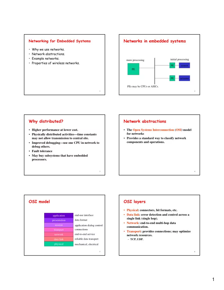
Networks in embedded systems
PE PE sensor PE actuator initial processing more processing PEs may be CPUs or ASICs.
3
Why distributed?
- Higher performance at lower cost.
- Physically distributed activities---time constants
may not allow transmission to central site.
- Improved debugging---use one CPU in network to
debug others.
- Fault tolerance
- May buy subsystems that have embedded
processors.
4
Network abstractions
- The Open Systems Interconnection (OSI) model
for networks
- Provides a standard way to classify network
components and operations.
5
OSI model
physical mechanical, electrical data link reliable data transport network end-to-end service transport connections presentation data format session application dialog control application end-use interface
6
OSI layers
- Physical: connectors, bit formats, etc.
- Data link: error detection and control across a
single link (single hop).
- Network: end-to-end multi-hop data
communication.
- Transport: provides connections; may optimize