1
play

1 Example : Example: Medical researchers have noted that adolescent - PDF document

Regression analysis is used to investigate whether there is a linear STAT E-150 relationship between two quantitative variables. Statistical Methods The variable we want to predict is the response variable ; the variable we use for this


  1. Regression analysis is used to investigate whether there is a linear STAT E-150 relationship between two quantitative variables. Statistical Methods The variable we want to predict is the response variable ; the variable we use for this prediction is the explanatory variable . Review of Linear Regression 2 If a linear relationship exists, we can create a model for the 
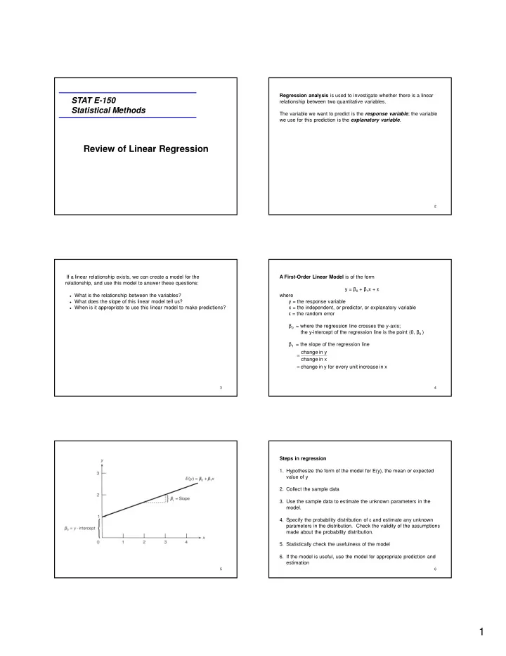
A First-Order Linear Model is of the form relationship, and use this model to answer these questions: y = � 0 + � 1 x + � � What is the relationship between the variables? where � What does the slope of this linear model tell us? y = the response variable � When is it appropriate to use this linear model to make predictions? x = the independent, or predictor, or explanatory variable � = the random error � 0 = where the regression line crosses the y-axis; the y-intercept of the regression line is the point (0, � 0 ) � 1 = the slope of the regression line change in y = change in x change in y for every unit increase in x = 3 4 Steps in regression 1. Hypothesize the form of the model for E(y), the mean or expected value of y 2. Collect the sample data 3. Use the sample data to estimate the unknown parameters in the model. 4. Specify the probability distribution of � and estimate any unknown parameters in the distribution. Check the validity of the assumptions made about the probability distribution. 5. Statistically check the usefulness of the model 6. If the model is useful, use the model for appropriate prediction and estimation 5 6 1

  2. Example : Example: Medical researchers have noted that adolescent females are more likely Medical researchers have noted that adolescent females are more likely to deliver low-birthweight babies than are adult females. Because LBW to deliver low-birthweight babies than are adult females. Because LBW babies tend to have higher mortality rates, studies have been conducted babies tend to have higher mortality rates, studies have been conducted to examine the relationship between birthweight and the mother’s age. to examine the relationship between birthweight and the mother’s age. One such study is discussed in the article “Body Size and Intelligence in One such study is discussed in the article “Body Size and Intelligence in 6-Year-Olds: Are Offspring of Teenage Mothers at Risk?” (Maternal and 6-Year-Olds: Are Offspring of Teenage Mothers at Risk?” (Maternal and Child Health Journal [2009], pp. 847-856.) Child Health Journal [2009], pp. 847-856.) Which is the response variable? Which is the response variable? The child’s birthweight (in grams) Which is the independent (or predictor or explanatory) variable? Which is the independent (or predictor or explanatory) variable? The mother’s age 7 8 The following data is consistent with summary values given in the article, The first step in determining whether there is a linear relationship and with data published by the National Center for Health Statistics: between the variables is to create a scatterplot of the data, with the explanatory variable on the x-axis and the response variable on the y-axis. Observation 1 2 3 4 5 6 7 8 9 10 Maternal Age (in years) 15 17 18 15 16 19 17 16 18 19 Birthweight (in grams) 2289 3393 3271 2648 2897 3327 2970 2535 3138 3573 Since there is only one independent variable, our model is of the form E(y) = � 0 + � 1 x 9 10 Does there appear to be a linear relationship? Does there appear to be a linear relationship? The scatter diagram shows a positive linear relationship 11 12 2

  3. What does the scatterplot tell you about the strength and direction of What does the scatterplot tell you about the strength and direction of the linear relationship? Write your answer in the context of the the linear relationship? Write your answer in the context of the scenario. scenario. The scatter diagram shows that there is a fairly strong positive The scatter diagram shows that there is a fairly strong positive linear relationship between the two variables: as the mother’s linear relationship between the two variables: as the mother’s age increases, the child’s birthweight also increased. age increases, the child’s birthweight also increased. That is, higher birthweightsare associated with older mothers. That is, higher birthweights are associated with older mothers. 13 The Method of Least Squares We want the size of the residuals to be as small as possible; since some residuals are positive and some are negative, we square the If the data appears to show a linear relationship, the method of least residuals and minimize the squares. squares finds the line that best fits the data. We can find the vertical distance between the observed value of y and � ) � � ) = 0 and �������� the predicted value of y for each value of x. This difference is called the The Least Squares line is the one where �������� residual : is minimized. The equation of the least squares line is y = � 1 x + � 0 Residual = observed value - predicted value � y y ε = − ε = − ε = − ε = − 15 16 The idealized regression line is E(y) = � 1 x + � 0 ; this model places the But since not all values of y will be on the line, for each data point (x, y) there is an error, ε , where ε = y - � y . mean of the distribution of y for each value of x on the line: So we now have the equation y = � 1 x + � 0 + � 17 18 3

  4. We will make these assumptions about the probability distribution The Standard Error for the Slope for the error, � : SE(b 1 ) indicates how much the slope varies from sample to sample. • The probability distribution of ε has a mean of 0 • The probability distribution of ε has a constant variance for all s values of x SE(b ) = e 1 n -1 s ⋅ ⋅ • The probability distribution of ε is approximately normal ⋅ ⋅ x • The errors associated with any two different observations are SE(b 1 ) will be smaller when independent. • s e , the standard deviation of the residuals, is smaller, indicating less scatter and a stronger relationship between x and y • n is larger • s x is larger, indicating a more stable regression with a broader range of x-values 19 20 Inferences about the slope � 1 The Sampling Distribution for Regression Slopes When the assumptions about the error, � , are met, the standardized To see if there is an association between x and y, we test the estimated regression slope, hypotheses H 0 : � 1 =0 b � − − − − 1 1 t = = = = H a : � 1 � 0 SE(b ) 1 � b b 0 b − − − − − − − − follows a Student’s t-model with n-2 degrees of freedom. using the test statistic t 1 1 1 1 = = = = = = = = = = = = SE(b ) SE(b ) SE(b ) 1 1 1 with n-2 degrees of freedom s We estimate the standard error with e , SE(b ) = 1 n -1 s ⋅ ⋅ ⋅ ⋅ x � � � � ˆ 2 (y - y) where s = e n - 2 n is the number of data values, and s x is the standard deviation of the x-values. 21 22 Assumptions for the model and the errors: 1. Linearity Assumption 3. Equal Variance Assumption: Straight Enough Condition: does the scatterplot appear linear? the variability of y should be about the same for all values of x � Check the residuals to see if they appear to be Does The Plot Thicken? Condition: randomly scattered Does the scatterplot show a constant spread about the line? � Check the residuals for any patterns Quantitative Data Condition: Is the data quantitative? 2. Independence Assumption: 4. Normal Population Assumption: the errors must be mutually independent the errors follow a Normal model at each value of x Randomization Condition: the individuals are a random sample Nearly Normal Condition: � Check the residuals for patterns, trends, clumping � Look at a histogram or NPP of the residuals 23 24 4

Download Presentation
Download Policy: The content available on the website is offered to you 'AS IS' for your personal information and use only. It cannot be commercialized, licensed, or distributed on other websites without prior consent from the author. To download a presentation, simply click this link. If you encounter any difficulties during the download process, it's possible that the publisher has removed the file from their server.

Recommend


More recommend