[PDF] - 1 SciVis Examples (2) Medicine Flow data sketch from Leonardo Da PDF Document

SLIDE 1

1 Introduction to Scientific Visualization

Stefan Bruckner

Simon Fraser University / Vienna University of Technology

Visualization – Definition

visualization: to form a mental vision, image,

r picture of (something not visible or present to

the sight, or of an abstraction); to make visible to

the mind or imagination

[Oxford Engl. Dict., 1989]

Stefan Bruckner 1

tool to enable a user insight into data

“The purpose of computing is insight, not numbers.”

[R. Hamming, 1962]

Visualization – Goals Visualization, …

… to explore

Nothing is known, Vis used for data exploration

… to analyze

Stefan Bruckner 2

y

There are hypotheses, Vis used for verification or falsification

… to present

“everything” known about the data, Vis used for communication of results

?! ?! Visualization – Areas Three major areas

Volume Visualization Flow

Scientific Visualization inherent spatial reference

Stefan Bruckner 3

Visualization Information Visualization

2D/3D nD usually no spatial reference InfoVis vs. SciVis N-dimensional vs. 2/3-dimensional

SciVis can be N-dimensional too (time series, simulation data, …)

Abstract data vs. spatial data

InfoVis data may also have spatial attributes InfoVis data may also have spatial attributes (country, state, …)

Discrete data vs. continuous data

InfoVis data may be sampled from a continuous domain

Stefan Bruckner 4

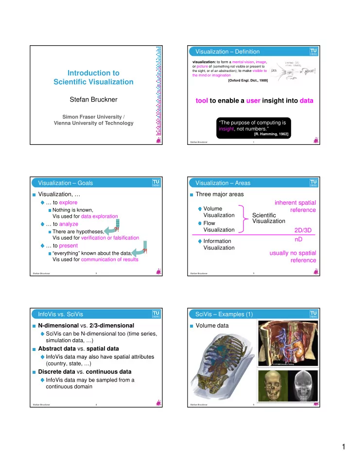
SciVis – Examples (1) Volume data

Stefan Bruckner 5

SLIDE 2

2 SciVis – Examples (2) Flow data

Stefan Bruckner 6

Medicine

Stefan Bruckner 7

sketch from Leonardo Da Vinci‘s anatomical notebooks medical illustrations by Clarice Ashworth Francone

Cartography

Stefan Bruckner 8

isolines to visualize compass deviations wind flow visualization Meteorology map with iso-pressure lines

Stefan Bruckner 9

weather fronts map for pilots Experimental Flow Investigation Fixation of tufts, ribbons on ...

aircraft in wind tunnels ship hull in fluid tanks

Stefan Bruckner 10

Introduction of smoke particles (in wind tunnel) Introduction of dye (in fluids) Visualization Scenarios complexity,

tech. demands

interactive steering

Stefan Bruckner 11

benefits, possibilities passive visualization interactive visualization

SLIDE 3

3 Visualization Pipeline Acquisition Enhancement Data are given Data are processed

Stefan Bruckner 12

Mapping Rendering Data are processed Data are mapped to, e.g., geometry Images generated Data Focus of visualization, everything is centered around the data Driving factor (besides user) in choice and attribution of the visualization technique Important questions

Stefan Bruckner 13

Important questions

In what domain are the data given? (data space) What is the type of data? (data characteristics) Which representation makes sense?

Data Space vs. Data Characteristics 1D 2D 3D 1D y=f(x) spatial curve x(t)

data characteristics ace

Stefan Bruckner 14

2D 3D 2D flow v(x) scalar field d(x) 3D flow v(x)

data spa

Grids – General Information Important questions

Which data organization is optimal? Where do the data come from? Is there a neighborhood relationship? How is the neighborhood information stored?

Stefan Bruckner 15

How is the neighborhood information stored? How is navigation within the data possible? Calculations with the data possible ? Are the data structured?

Grid - Types Cartesian grid Curvilinear grid

dx dy } } x[0,0] x[0,ymax] x[xmax,0]

Unstructured grid Scattered data

Stefan Bruckner 16

[ , ] x[0] x[1] e[0] c[0]

Grids - Survey struc- tured grids block-structu

rtho-

gonal grids equi- dist. grids cartesian grids (dx=dy) regular id (d d )

Stefan Bruckner 17

unstructured grids hybrid grids miscell. rde grids curvi-linear grids rectilinear grids grids (dxdy)

SLIDE 4

4 Volume Visualization VolVis = visualization of volume data

Mapping 3D2D

Volume data

3D1D data Scalar data 3D data space space filling Scalar data, 3D data space, space filling

User goals

Gain insight in 3D data Structures of special interest + context

Stefan Bruckner 18

Volume Data Medicine

CT, MRI, PET, Ultrasound

Biology

Confocal microscopy Confocal microscopy, histological cuts

Geology

Seismic surveys

Material testing

Industrial CT

Stefan Bruckner 19

3D Data Space Cartesian/regular grid

Most common, e.g., CT/MRI scans

Curvilinear/unstructured grid

Less frequently, e.g., simulation data

Stefan Bruckner 20

Concepts and Terms sampled data (measurement) analytical data (modelling) voxel space geometric surfaces

iso-surfacing

Stefan Bruckner 21

voxel space (discrete) geometric surfaces (analytic) pixel space (discrete)

voxelization surface rendering (direct) volume rendering

Volume Rendering (1) Deals with the visual representation of 3D functions Frequently, but not exclusively, functions are

Stefan Bruckner 22

y, scalar-valued Often aquired using sampling (e.g., medical domain) Volume Rendering (2) Initially volumes were visualized using two- dimensional cuts Extraction of surface geometry for isosurfaces in the volume (e.g. Marching Cubes [Lorensen and Cline 1987]) ]) Volume rendering introduced almost simultaneously by [Levoy 1988] and [Drebin et

al. 1988]

Stefan Bruckner 23

SLIDE 5

5 Surface vs. Volume Rendering Surface rendering

Indirect volume visualization Intermediate representation: iso-surface Pros: Less memory, fast rendering

Volume rendering

Stefan Bruckner 24

Volume rendering

Direct volume visualization Usage of transfer functions Pros: illustrate the interior, semi-transparency

Volume Ray Casting Volume: 1D value defined in 3D f(x)R1, xR3 Ray: Half-line r(t)R3, tR1>0 ( ) , Intensity profile: values along a ray f(r(t))R1, tR1>0 Image plane: starting points of rays

Stefan Bruckner 25

Pipeline – Overview

reconstruction classification reconstruction classification

volume rendering pipeline

data set final image

c ass cat o shading compositing c ass cat o shading compositing

Pipeline – Reconstruction

reconstruction classification reconstruction classification

volume rendering pipeline

data set final image

c ass cat o shading compositing c ass cat o shading compositing

Reconstruction (1) Usually volume data sets are given as a grid

f discrete samples

For rendering purposes, we want to treat them as continuous three-dimensional functions We need to choose an appropriate We need to choose an appropriate reconstruction filter Requirements: high-quality reconstruction, but small performance overhead

Stefan Bruckner 28

image plane

Reconstruction (2)

data set eye

SLIDE 6

6 Reconstruction (3)

cell cell

sample point sample point

Stefan Bruckner 30

cell cell

voxel voxel

Trilinear Interpolation Simple extension of linear interpolation to three dimensions Advantage: current GPUs automatically do trilinear interpolation of 3D textures

Stefan Bruckner 31

Other Reconstruction Filters If very high quality is required, more complex reconstruction filters may be required Marschner-Lobb function is a common test signal to evaluate the quality of reconstruction filters [Marschner and Lobb 1994] [ ] The signal has a high amount of its energy near its Nyquist frequency Makes it a very demanding test for accurate reconstruction

Stefan Bruckner 32

Comparison of Reconstruction Filters (1) Marschner-Lobb test signal (analytically evaluated)

Stefan Bruckner 33

Comparison of Reconstruction Filters (2) Trilinear reconstruction of Marschner-Lobb test signal

Stefan Bruckner 34

Comparison of Reconstruction Filters (3) Cubic reconstruction of Marschner-Lobb test signal

Stefan Bruckner 35

SLIDE 7

7 Comparison of Reconstruction Filters (4) B-Spline reconstruction of Marschner-Lobb test signal

Stefan Bruckner 36

Comparison of Reconstruction Filters (5) Windowed sinc reconstruction of Marschner- Lobb test signal

Stefan Bruckner 37

Comparison of Reconstruction Filters (6) Marschner-Lobb test signal (analytically evaluated)

Stefan Bruckner 38

Pipeline – Classification

reconstruction classification reconstruction classification

volume rendering pipeline

data set final image

c ass cat o shading compositing c ass cat o shading compositing

Classification (1) Projecting a 3D data set onto a 2D image is problematic Not all information contained in the volume is relevant to the user Classification allows the user to extract the Classification allows the user to extract the important parts of the data

Stefan Bruckner 40

During Classification the user defines the appearence of the data

Which parts are transparent? Which parts have which color?

Classification (2)

SLIDE 8

8 During Classification the user defines the appearence of the data

Which parts are transparent? Which parts have which color?

The user defines a transfer function Classification (3) The user defines a transfer function

color RGB

pacity A

scalar S

Transfer Functions (1)

real-time update of the transfer function important

Transfer Functions (2) Classification Order (1) Classification can occur before or after reconstruction Pre-interpolative: classify all data values and then interpolate between RGBA-tuples Post-interpolative: interpolate between Post interpolative: interpolate between scalar data values and then classify the result

Stefan Bruckner 45

Classification Order (2)

al properties

interpolation

PRE-INTERPOLATIVE

al properties

POST-INTERPOLATIVE

ptic

data value

ptic

data value

interpolation

supersampling transfer function transfer function continuous data discrete data

scalar value alpha value

Classification Order (3)

post-interpolative classified data supersampling analytical solution pre-interpolative transfer function

SLIDE 9

9 Classification Order (4)

same transfer function, resolution, and sampling rate

pre-interpolative post-interpolative

Classification Order (5)

pre-interpolative post-interpolative

same transfer function, resolution, and sampling rate

Pipeline – Shading

reconstruction classification reconstruction classification

volume rendering pipeline

data set final image

c ass cat o shading compositing c ass cat o shading compositing

Shading (1) Make structures in volume data sets more realistic by applying an illumination model Shade each sample in the volume like a surface Any model used in real-time surface graphics Any model used in real time surface graphics suitable Common choice: Blinn-Phong illumination model

Stefan Bruckner 51

Shading (2) Local illumination, similar to surface lighting

Lambertian reflection light is reflected equally in all directions Specular reflection light is reflected scattered around the direction of perfect reflection

shaded volume rendering unhaded volume rendering

Shading (3)

Stefan Bruckner 53

SLIDE 10

10 Gradient Estimation (1) Normalized gradient vector of the scalar field is used to substitute for the surface normal The gradient vector is the first-order derivative

f the scalar field

partial derivative p in x-direction partial derivative in y-direction partial derivative in z-direction

We can estimate the gradient vector using finite differencing schemes, e.g. central differences: Gradient Estimation (2) Noisy data may require more complex estimation schemes Gradient Magnitude Magnitude of gradient vector can be used to measure the “surfaceness” of a point

Strong changes  high gradient magnitude Homogenity  low gradient magnitude

Applications Applications

Use gradient magnitude to modulate opacity

f sample

Interpolate between unshaded and shaded sample color using gradient magnitude as weight

Stefan Bruckner 56

Pipeline – Compositing

reconstruction classification reconstruction classification

volume rendering pipeline

data set final image

c ass cat o shading compositing c ass cat o shading compositing

Compositing (1) So far, everything discussed applies to single sample points along a viewing ray How to subsequent sample when traversing the ray? Common models Common models

Maximum Intensity Projection Emission-Absorption Model

Stefan Bruckner 58

Maximum Intensity Projection (1) Always display the maximum value along a viewing ray Motivation: visualization of contrast-enhanced tomographic scans Parameterless rendering, very common in medical domain

59 Stefan Bruckner

SLIDE 11

11 Maximum Intensity Projection (2) Probem: loss of spatial relationships between different structures

Stefan Bruckner 60

Emission-Absorption Model (1) Conventional volume rendering uses an emission-absorption model Scattering effects are usually ignored due to high computational complexity For each pixel on the image plane a the ray For each pixel on the image plane, a the ray integral has to be solved For each step along he viewing ray, perform accumulate RGBA from transfer function

Stefan Bruckner 61

in-scattering

increase

emission

Emission-Absorption Model (2)

decrease

absorption

ut-scattering

Ray Integration (1)

image plane data set eye

How do we determine the radiant energy along the ray?

Physical model: emission and absorption, no scattering

viewing ray

Ray Integration (2)

absorption along the distance s - s

~

active emission at point s

~

Every point along the viewing ray emits additional radiant energy

image plane

Numerical Solution (1)

data set eye

SLIDE 12

12 Numerical Solution (2)

can be computed recursively

radiant energy

bserved at position i

radiant energy emitted at position i radiant energy

bserved at position i–1

absorption at position i

Numerical Solution (2)

back-to-front compositing front-to-back compositing early ray termination: stop the calculation when

Flow Visualization FlowVis = visualization of flows

Visualization of change information

Flow data

nDnD data, 1D2 /2D2/nD2 (models), 2D2/3D2 Vector data (nD) in nD data space Vector data (nD) in nD data space Steady vs. time-dependent flow

User goals

Overview vs. details (with context)

Stefan Bruckner 69

Flow Data (1) Simulation

Flow space modelled with grid FEM (finite elements method), CfD (computational fluid dynamics)

Measurements

Stefan Bruckner 70

Measurements

Optical methods + pattern recognition, e.g.: PIV (particle image velocimetry)

Models

Differential equation systems dx/dt

Flow Data (2)

Stefan Bruckner 71

SLIDE 13

13 Flow Data (3) experiment

Stefan Bruckner 72

simulation Direct Flow Visualization Grid of arrows to visualize flow directions Normalized arrows vs. scaling with velocity g y Quite effective in 2D, problematic in 3D Sometimes limited expressivity (temporal component missing)

Stefan Bruckner 73

Geometric Flow Visualization Idea: follow the flow in time (integration) to extract the path of a particle

Stefan Bruckner 74

Streamlines – Theory

Flow data v: derivative information

dx/dt = v(x)

spatial points xRn, flow vectors vRn, time tR

Streamline s: integration over time, also called trajectory, solution, curve also called trajectory, solution, curve

s(t) = s0 + 0utv(s(u)) du

seed point s0, integration variable u

Difficulty: result s also in the integral, analytical solution usually impossible

Stefan Bruckner 75

Streamlines – Practice (1)

Solve using numerical integration techniques Assume that locally the solution is approximately linear E ler integration Euler integration

si+1 = si + dt· v(si) Follow the current flow vector v(si) from the current streamline point si for a short time (dt)

Stefan Bruckner 76

Streamlines – Practice (2) Accuracy of results is strongly dependent on step size dt

Stefan Bruckner 77

SLIDE 14

14 Streamlines – Placement (1) Seed fill with streamlines to achieve equal density

Stefan Bruckner 78

Streamlines – Placement (2) Variations of distance in relation to image width

3% 6% 1.5%

Stefan Bruckner 79

Illuminated Streamlines Illuminated 3D curves improve perception

Stefan Bruckner 80

Stream Surfaces Natural extension of streamlines to 3D Surfaces which are tangential to the vector field everywhere y Challenges related to

cclusion and visual

complexity

Stefan Bruckner 81

Flow Volumes Volumetric equivalents

f streamlines, subset of

a 3D flow domain is traced in time Can be visualized with direct volume rendering methods

Stefan Bruckner 82

Unsteady Flow Path line

Trajectory of an individual particle in the fluid flow

Timeline

Joins the positions of particles released at the Joins the positions of particles released at the same instant in time

Streak line

Connects particles that have passed through a certain point in space

Stefan Bruckner 83

SLIDE 15

15 Texture-based Flow Visualization Idea: exploit visual correlations to provide a dense visualization of the flow

Stefan Bruckner 84

Line Integral Convolution Calculation of a texture value

look at streamline through point

flow data streamline integration l ti

filter white noise along streamline

Stefan Bruckner 85

white noise LIC texel convolution results in

Line Integral Convolution – Examples (1)

laminar flow

Stefan Bruckner 86

turbulent flow

Line Integral Convolution – Examples (2)

Stefan Bruckner 87

Line Integral Convolution on Surfaces

Stefan Bruckner 88

Texture Advection – Unsteady Flows

Stefan Bruckner 89

SLIDE 16

16 Feature-based Flow Visualization Extract and visualize the abstract structure

f a flow

Stefan Bruckner 90

Different elements

Checkpoints, defined through v(x)=0 Cycles, defined through sx(t+T)=sx(t) Connecting structures (separatrices, etc.)

Vector Field Topology Critical points can be classified by the Eigenvalues of the Jacobian

R = real components, I = imaginary components

Stefan Bruckner 91

Glyphs/Icons Local/ topological properties

Stefan Bruckner 92

Examples (1) Topology of a hurricane simulation

Stefan Bruckner 93

Examples (2) Visualization of flow past a circular cylinder using critical points and saddle connectors

Stefan Bruckner 94